Learn R Programming (Tutorial & Examples) | Free Introduction

So without too much talk, let’s get started…

What is R Programming & What is it Used for?

R is a programming language and software that is becoming increasingly popular in the disciplines of statistics and data science.

R is a dialect of the S programming language and was developed by Ross Ihaka and Robert Gentleman in the year 1995. A stable beta version was released in the year 2000.

The R software is completely free and gets developed collaboratively by its community (open-source software) – every R user can publish new add-on packages.

The open-source ideology of R programming reflects a huge contrast compared to most traditional programming environments (e.g. SAS, SPSS, Stata etc.), where the software development is in the hands of a paid development team.

Why You Should Learn the R Programming Language (Pros & Cons)

There are many reasons why you should – or should not – learn R! The list below provides an overview of some of the most important advantages and disadvantages of the R programming language.

The pros:

✅ R is free

✅ R’s popularity is growing – More and more people will use it

✅ Almost all statistical methods are available in R

✅ New methods are implemented in add-on packages quickly

✅ Algorithms for packages and functions are publicly available (transparency and reproducibility)

✅ R provides a huge variety of graphical outputs

✅ R is very flexible – Essentially everything can be modified for your personal needs

✅ R is compatible with all operating systems (e.g. Windows, MAC, or Linux)

✅ R has a huge community that is organized in forums to help each other (e.g. Stack Overflow)

✅ R is fun 🙂

The cons:

❌ Relatively high learning burden at the beginning (even though it’s worth it)

❌ No systematic validation of new packages and functions

❌ No company in the background that takes responsibility for errors in the code (this is especially important for public institutes)

❌ R is almost exclusively based on programming (no extensive drop-down menus such as in SPSS)

❌ R can have problems with computationally intensive tasks (only important for advanced users)

You might already have noticed that I’m a big fan of R, so in my opinion it’s definitely one of the best programming languages to master! Once you know the basics, this programming language will become easier and easier to use.

R & RStudio Interface Explained

It is important to understand the difference between R and RStudio:

• R is the programming language. You may run your R programs directly via the command prompt or terminal.
• RStudio is an Integrated Development Environment (IDE), i.e. an interface for the R programming language that makes it easier to write and execute scripts.

If you are an advanced programmer, or if you are running R on a server, you might want to use R without the RStudio interface. However, nowadays almost everybody uses the RStudio interface to program in R, and I highly recommend you to do so as well.

Downloading and installing R and RStudio is pretty straightforward. You can download the R programming language here, and you can download RStudio here.

Make sure to install R before RStudio, because otherwise the RStudio installation will show a warning message.

Once you have installed R and RStudio, you basically never have to open R again. All the future work will be done directly in RStudio.

Let’s have a look at the different components of the RStudio interface. Below, you can see a screenshot of a typical RStudio session:

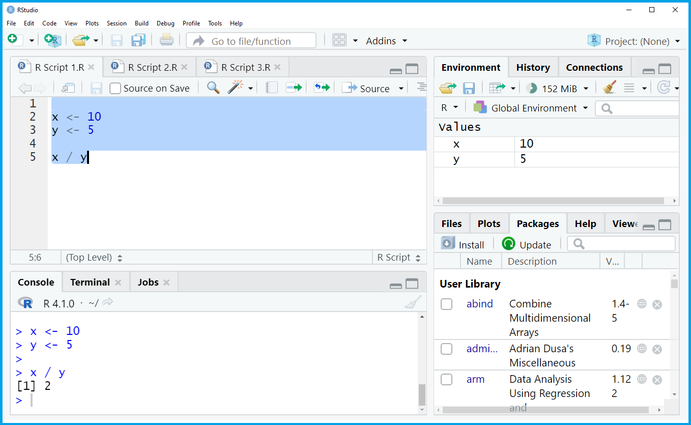
As you can see, the RStudio interface is basically split into four different panels:

In the remaining part of this tutorial, I’ll show how to use these different panels of the RStudio IDE in action.

Let’s dive into the R programming examples!

Data Manipulation in R

Before we jump into the programming examples: I have published an extensive introduction tutorial to the R programming language as a 10K subscriber special on the Statistics Globe YouTube channel.

This tutorial illustrates the following R programming examples in video format. In case you prefer to learn by watching and listening instead of reading, you may check out the free video course below:

The R code used in this video can be found here.

However, you will also find all the R programming code as well as detailed explanations on this code below.

So let’s move on to the first section – data manipulation in R!

Data manipulation is often the very first step when creating a new program in R. It is usually necessary as a preparation for the visualization and analysis of the data.

For this, you first have to know that the R programming language provides different types of data.

In the first part of this tutorial, I’ll show how to create your own data in R (later, you will also learn how to import external data into R).

Let’s do this!

Creation of Different Data Structures

The R programming code below shows how to create a vector object in R. Vectors are sequences of data elements of the same class.

To create such a vector object, we have to apply the c function. Within the c function, we have to specify the vector elements that our vector should contain:

vec_1 <- c(1, 1, 5, 3, 1, 5)                                              # Create vector object
vec_1                                                                     # Print vector object
# [1] 1 1 5 3 1 5

Have a look at the previous R code and its output. As you can see, we have created a new vector object called vec_1. This vector contains six integer elements, i.e. the numbers 1, 1, 5, 3, 1, and 5.

The next data type that I want to show you are data frames. Data frames are two-dimensional objects with a certain number of rows and columns.

Let’s create such a data frame in R:

data_1 <- data.frame(x1 = c(7, 2, 8, 3, 3, 7),                            # Create data frame
                     x2 = c("x", "y", "x", "x", "x", "y"),
                     x3 = 11:16)
data_1                                                                    # Print data frame

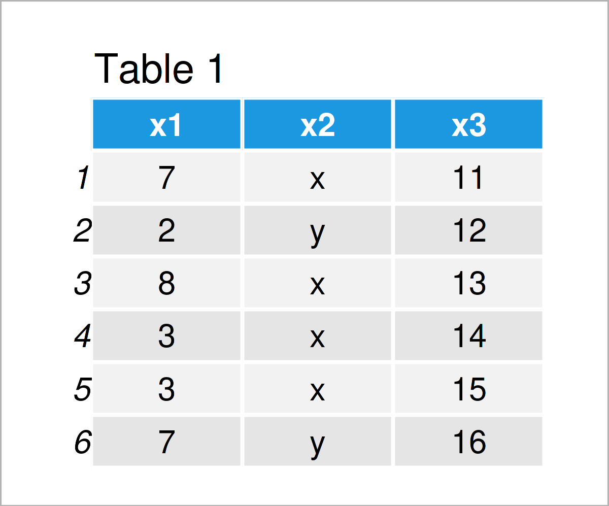
In Table 1 it is shown that we have created a new data frame called data_1. This data frame consists of six rows and the three columns (or variables) x1, x2, and x3. The columns x1 and x3 contain numbers; the column x2 contains characters.

The third type of data object that I want to explain are lists. Lists contain different list elements (or items), and each of these list elements can contain a different data type.

For instance, the following code creates a list with three list elements. The first list element contains a range from 1 to 5, the second list element contains our vector object vec_1, and the third list element contains our data frame data_1:

list_1 <- list(1:5,                                                       # Create list
               vec_1,
               data_1)
list_1                                                                    # Print list
# [[1]]
# [1] 1 2 3 4 5
# 
# [[2]]
# [1] 1 1 5 3 1 5
# 
# [[3]]
#   x1 x2 x3
# 1  7  x 11
# 2  2  y 12
# 3  8  x 13
# 4  3  x 14
# 5  3  x 15
# 6  7  y 16

In summary: The previous code has illustrated three of the most common data structures in R. The graphic below summarizes the main differences between these data types:

Note that the R programming language provides many other data types (e.g. arrays, matrices, tibbles, data.tables etc.) that I haven’t shown yet.

However, the three data types vector, data frame, and list already provide you with a good basis for the following examples.

Let’s move on to the next data manipulation section!

Handling Data Classes

In the previous section, you may already have noticed that we have dealt with different data classes (i.e. numeric and character).

Data classes are a critical topic when programming in R, since each data class is used for different tasks.

The following code explains some of the most important data classes in R.

Let’s first check the data class of the vector object that we have created at the beginning of the data manipulation section. To check the class, we can use the class function as shown below:

class(vec_1)                                                              # Check class of vector elements
# [1] "numeric"

As you can see, RStudio has returned “numeric” to the console, i.e. our vector object vec_1 has the class numeric. The numeric class is used for numbers.

Another class that we have already used when we created the data frame in the previous section is the character class.

Let’s create a vector object containing character elements:

vec_2 <- c("a", "b", "a", "c")                                            # Create character vector
vec_2                                                                     # Create character vector
# [1] "a" "b" "a" "c"

As you can see based on the previous console output, the character class is used for text elements (also called character strings).

Based on the quotes around the letters, you can already see that we are dealing with characters. However, we can also apply the class function to our new vector object to return its class to the RStudio console:

class(vec_2)                                                              # Check class of vector elements
# [1] "character"

Our guess was confirmed – The vector object vec_2 has the character class.

Another important R programming class are factors. Similar to characters, factor can contain letters and numbers. However, the difference compared to characters is that each element has a meaning.

Let’s illustrate that by creating our own factor vector:

vec_3 <- factor(c("gr1", "gr1", "gr2", "gr3", "gr2"))                     # Create factor vector
vec_3                                                                     # Print factor vector
# [1] gr1 gr1 gr2 gr3 gr2
# Levels: gr1 gr2 gr3

The previous output shows the values in our factor vector as well as another output row called “Levels”. The levels of a factor object reflect all possible values a certain factor can have.

In other words: A factor has specific nominal categories and each of these categories has a particular meaning.

An example for a factor variable would be country names. Each country name corresponds to a specific geographical area, and hence we could cluster each observation in a data set by its country.

For completeness, let’s apply the class function to our vector to return its class to the RStudio console:

class(vec_3)                                                              # Check class of vector elements
# [1] "factor"

No surprising news – Our vector object has the factor class.

The figure below summarizes the ideas of the previous part of the tutorial:

As illustrated above, the class of a data object is essential for the further handling of this data object. For that reason, we sometimes might want to convert certain data objects or data frame columns to a different class.

The following R syntax shows how to perform such a data class transformation in R. More precisely, we use the as.character function to convert the factor vector vec_3 to the character class:

vec_4 <- as.character(vec_3)                                              # Convert factor to character
vec_4                                                                     # Print updated vector
# [1] "gr1" "gr1" "gr2" "gr3" "gr2"

The previous output has created a new vector object called vec_4, which contains the same elements as the vector vec_3, but with a different data class. Let’s check this:

class(vec_4)                                                              # Check class of updated vector elements
# [1] "character"

As you can see, we have switched the class from factor to character.

Add & Remove Columns & Rows of a Data Set

So far, we have created different data objects, and we have manipulated the data classes of these data objects.

The next part of the tutorial shows how to add or remove certain values to and from an already existing data object.

The first piece of code demonstrates how to add a new column to a data set.

The code is split into three different rows: First, we replicate our data frame data_1 that we have created at the beginning of the data manipulation section. We do this in order to keep an original version of our input data frame data_1.

In the second line, we use the $ operator to assign the values stored in the vector object vec_1 as a new column called x4 to our data frame. Note that the vector object vec_1 needs to have the same number of elements as the number of rows in our data set.

Finally, we print the updated data frame to the RStudio console by running the third line of the following piece of code.

data_2 <- data_1                                                          # Create duplicate of data frame
data_2$x4 <- vec_1                                                        # Add new column to data frame
data_2                                                                    # Print updated data frame

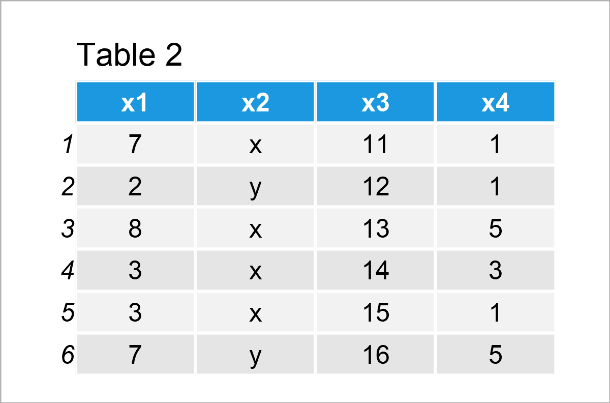
Table 2 shows the output of the previous R programming syntax – We have constructed a new data frame called data_2 that contains the columns of the data set data_1 plus an additional column containing the values of the vector object vec_1.

It is also possible to use the R programming language to remove columns from a data frame.

The R code below uses the colnames function and a logical condition to drop the variable x2 from our data set:

data_3 <- data_2[ , colnames(data_2) != "x2"]                             # Remove column from data frame
data_3                                                                    # Print updated data frame

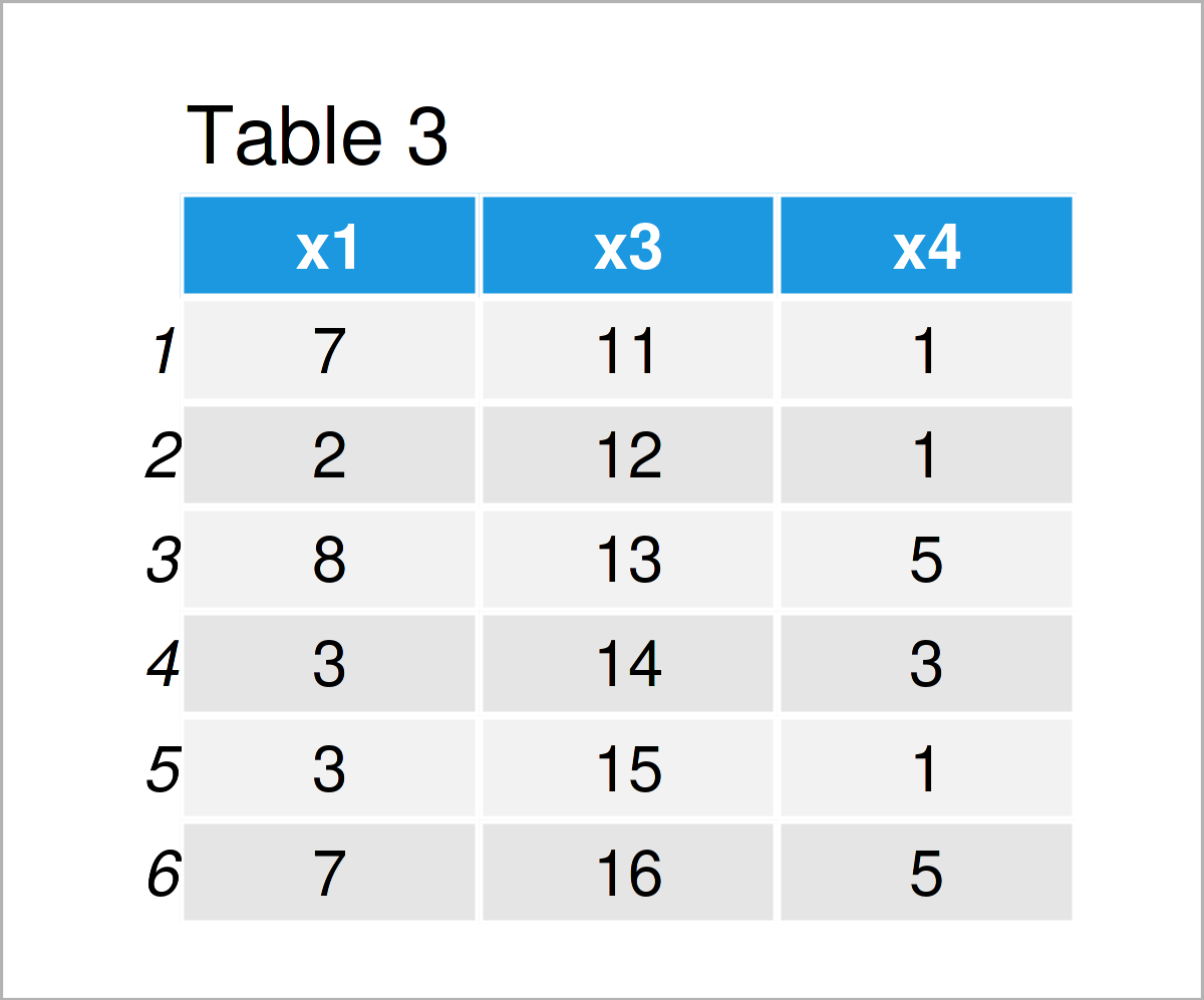
In Table 3 it is shown that we have created another data frame called data_3 using the previously shown R code. This data frame contains only the variables x1, x3, and x4. The variable x2 has been deleted.

When modifying the columns of a data frame, it often makes sense to rename the column names of the final data set.

Once again, we can use the colnames function:

data_4 <- data_3                                                          # Create duplicate of data frame
colnames(data_4) <- c("col_A", "col_B", "col_C")                          # Change column names
data_4                                                                    # Print updated data frame

After executing the previous R code the data frame shown in Table 4 has been created. As you can see, we have exchanged the column names by the new names “col_A”, “col_B”, and “col_C”.

Until now, we have adjusted the column structure of our data frame. However, it’s also possible to modify the rows of a data frame.

The R syntax below illustrates how to add a new row at the bottom of a data set. For this task, we can apply the rbind function:

data_5 <- rbind(data_3, 101:103)                                          # Add new row to data frame
data_5                                                                    # Print updated data frame

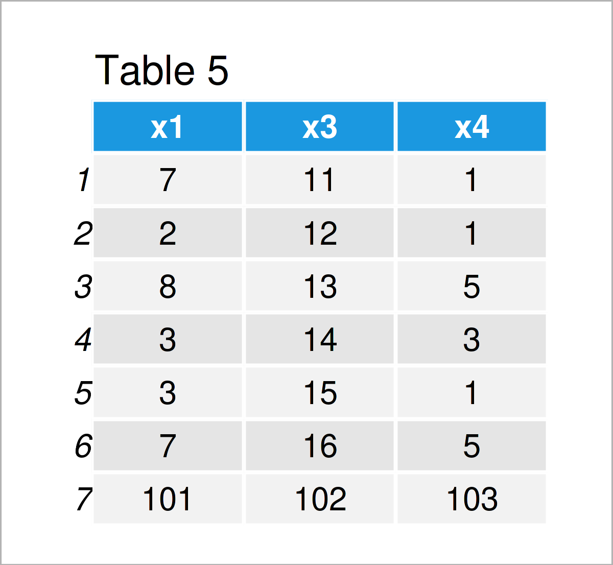
As shown in Table 5, the previous R programming code has created a new data frame called data_5 where the sequence from 101 to 103 has been added as an additional row at the bottom.

We can also delete certain rows from a data frame.

The following example drops rows based on a logical condition, i.e. we only want to keep rows where the value in the column x1 is larger than 3:

data_6 <- data_5[data_5$x1 > 3, ]                                         # Remove rows from data frame
data_6                                                                    # Print updated data frame

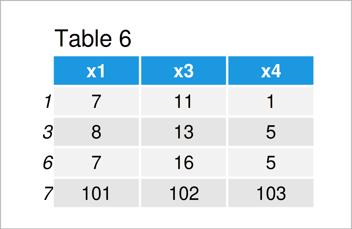
By executing the previous R programming code, we have created Table 6, i.e. a subset of the rows of our input data frame data_5.

Merge Multiple Data Frames

In the previous part of this tutorial, you have already learned how to append a vector object as a single new column horizontally to a data frame.

However, sometimes you might want to concatenate multiple data frames coming from different data sources into a single data set.

This is especially the case when the information about certain observations is stored in different data sources.

The process of combining these data is often called “merge” or “join”.

The following example demonstrates how to conduct such a merge in the R programming language.

For this example, we first have to create two new data frames:

data_7 <- data.frame(ID = 101:106,                                        # Create first data frame
                     x1 = letters[1:6],
                     x2 = letters[6:1])
data_7                                                                    # Print first data frame

data_8 <- data.frame(ID = 104:108,                                        # Create second data frame
                     y1 = 1:5,
                     y2 = 5:1,
                     y3 = 5)
data_8                                                                    # Print second data frame

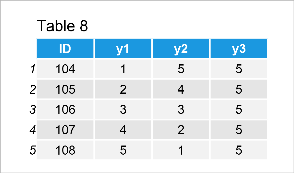
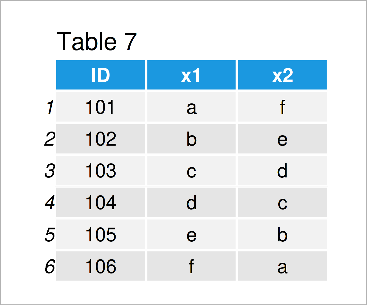
Our two example data frames are shown in Tables 7 and 8. As you can see, both of these data frames contain an ID column, but different other variables (i.e. x1 and x2 in the first data frame and y1, y2, and y3 in the second data frame).

If we want to merge these data into a single data set, we can use the merge function as shown below:

data_9 <- merge(x = data_7,                                               # Merge two data frames
                y = data_8,
                by = "ID",
                all = TRUE)
data_9                                                                    # Print merged data frame

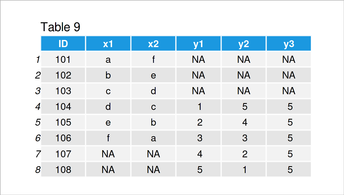
As shown in Table 9, the previous R syntax has created a union between our two input data frames.

Note that the previous R code has performed a full outer join, i.e. all rows of both data frames have been kept, no matter if the ID was existent in both data frames. Please have a look here, in case you want to learn more about different types of joins.

Replace Values in Vectors & Data Frames

In the previous examples I have demonstrated how to add or remove entire columns and rows. This section, in contrast, shows how to replace only specific data cells in a data object.

In the code snippet below, I illustrate how to exchange a certain value in a vector object by a new value.

To be more specific, the R code below first duplicates our example vector vec_1 in a new vector object called vec_5. Then, we use a logical condition to replace each occurrence of the value 1 by the value 99. Finally, we print the new vector to the RStudio console:

vec_5 <- vec_1                                                            # Create duplicate of vector
vec_5[vec_5 == 1] <- 99                                                   # Replace certain value in vector
vec_5                                                                     # Print updated vector
# [1] 99 99  5  3 99  5

Similar to the previous code snippet, we can also replace particular elements in a data frame.

The R syntax below shows how to substitute each appearance of the character “y” by the character string “new”:

data_10 <- data_1                                                         # Create duplicate of data frame
data_10$x2[data_10$x2 == "y"] <- "new"                                    # Replace values in column
data_10                                                                   # Print updated data frame

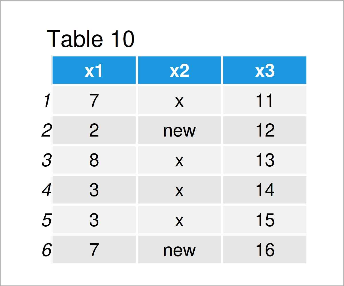
The output of the previous syntax is revealed in Table 10 – A new data frame where “y” was set to “new”.

Export & Import Data Sets

We have created many different data frames in this tutorial. To make these data frames accessible outside of R, we might want to export them to an external file on our computer.

This specific example explains how to export a data frame to a CSV file. However, we might use a similar syntax to create other types of files such as XLSX and TXT files.

In any case, we first have to specify the working directory where our file should be saved.

To identify the currently used working directory, we can use the getwd function:

getwd()                                                                   # Get current working directory
# [1] "C:/Users/Joach/Documents"

As you can see based on the previous output of the RStudio console, our current working directory is the Documents folder on my computer.

Let’s assume that we have a folder called my_directory on the desktop of our computer:

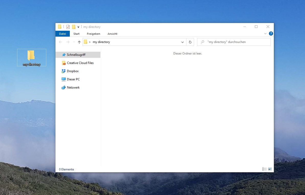
Then, we can set the working directory of the current R session to this folder using the setwd function as shown below:

setwd("C:/Users/Joach/Desktop/my directory")                              # Set new working directory

Let’s check the current working directory once again using the getwd command:

getwd()                                                                   # Get current working directory
# [1] "C:/Users/Joach/Desktop/my directory"

As you can see, we have changed the working directory to the folder on my desktop.

In the next step, we can apply the write.csv function to export a certain data frame as a CSV file to our working directory.

Within the write.csv function, we have to specify the name of the data frame that we want to save (i.e. data_10), and the name of the output file (i.e. “data_10.csv”). In addition, we also specify that we want to avoid printing row names to the exported CSV file.

write.csv(data_10,                                                        # Export data frame to CSV file
          "data_10.csv",
          row.names = FALSE)

After executing the R code above, our directory is updated:

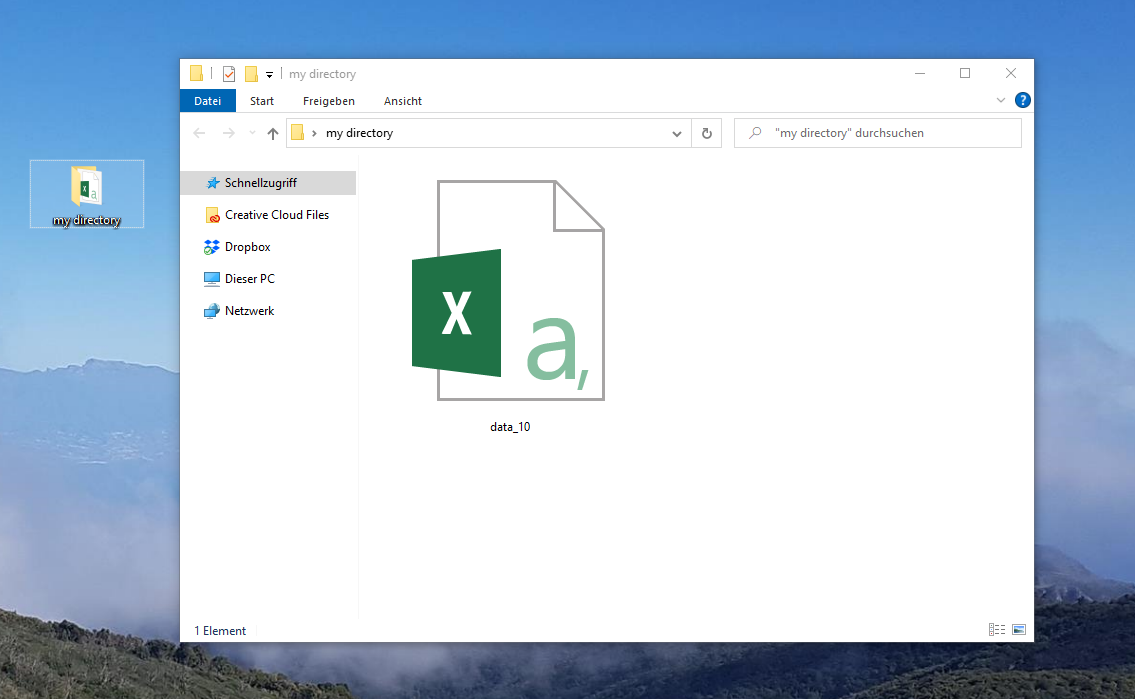
As you can see, we have written the data frame data_10 as a CSV file to our working directory.

In case we want to import this file to another R session, we can simply use the read.csv function as shown below:

data_11 <- read.csv("data_10.csv")                                        # Import data frame from CSV file
data_11                                                                   # Print imported data frame

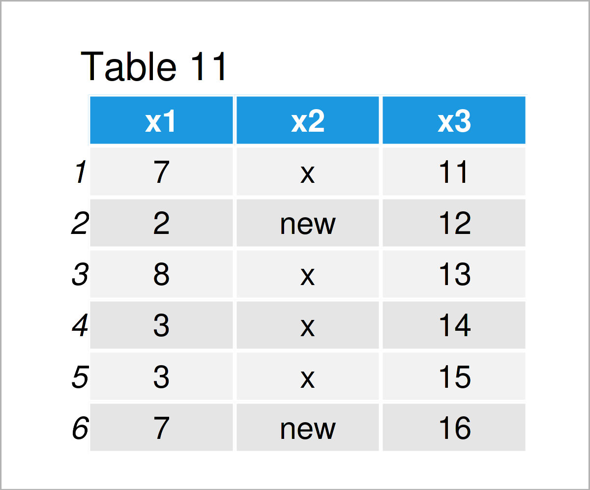
The output of the previous syntax is shown in Table 11: We have imported the CSV file “data_10.csv”, and we have stored this file as a new data frame object called data_11.

At this point of the tutorial, I want to stop talking about data manipulation and data wrangling in R.

In case you have any specific questions that have not been covered yet, you may type your question to the search mask at the top right of the menu bar on this website. I have published several hundreds of different articles on data manipulation already.

However, let’s move on to the visualization of our data in different types of graphics!

Creating Graphics in R

The capability to draw and modify graphics is an important requirement to a programming language – especially when it comes to a statistical analysis tool such as R.

Fortunately, the creation of different types of graphics is straightforward in the R programming language, and at the same time one of the major reasons why R is so powerful.

In the following section, I will show you how to create and adjust graphics to fit your own needs.

So keep on reading!

Creating Graphics Using Base R

The basic installation of the R programming language already provides amazing features for the creation of graphics in R.

In this subsection, I will show you how to create some of the most common types of graphs using Base R.

The data frames created in the previous data manipulation section are a bit too simple to show all the pretty graphical features of R, so let’s first load some more complex data into R.

The R programming language provides some preloaded data sets, and one of the most common ones is the iris data set that we can load by executing the following code:

data(iris)                                                                # Load iris data set
head(iris)                                                                # Print head of iris data set

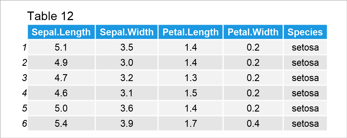
After executing the previous R syntax the data frame shown in Table 12 has been loaded. As you can see, the iris data set contains information on different flower species.

Enough talk about the data, let’s finally draw some plots!

One of the most common type of graphics are so-called scatterplots (or xy-plots), and we can draw such a scatterplot using the plot function.

Within the plot function, we have to specify the x-axis and the y-axis values. In the following syntax, we also specify the col argument to be equal to the Species column in our data to reflect the data points of each species by a different color.

plot(x = iris$Sepal.Length,                                               # Draw Base R scatterplot
     y = iris$Sepal.Width,
     col = iris$Species)

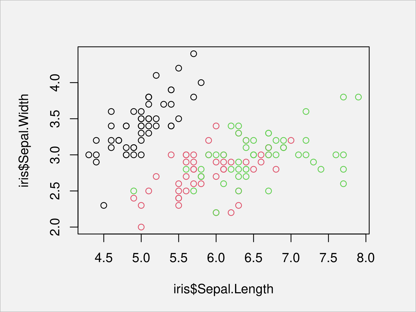
After executing the previous R programming syntax the scatterplot shown in Figure 1 has been drawn. As you can see, each species is reflected by a different color.

Another popular kind of graphics are kernel density plots.

We can draw a Base R density plot using the plot function in combination with the density function.

The following example code created a density plot of the iris column Sepal.Length:

plot(density(x = iris$Sepal.Length))                                      # Draw Base R density plot

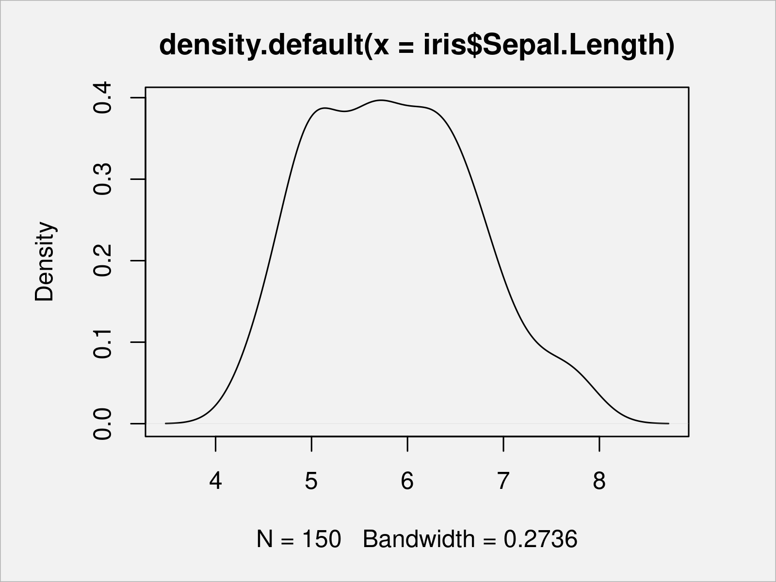
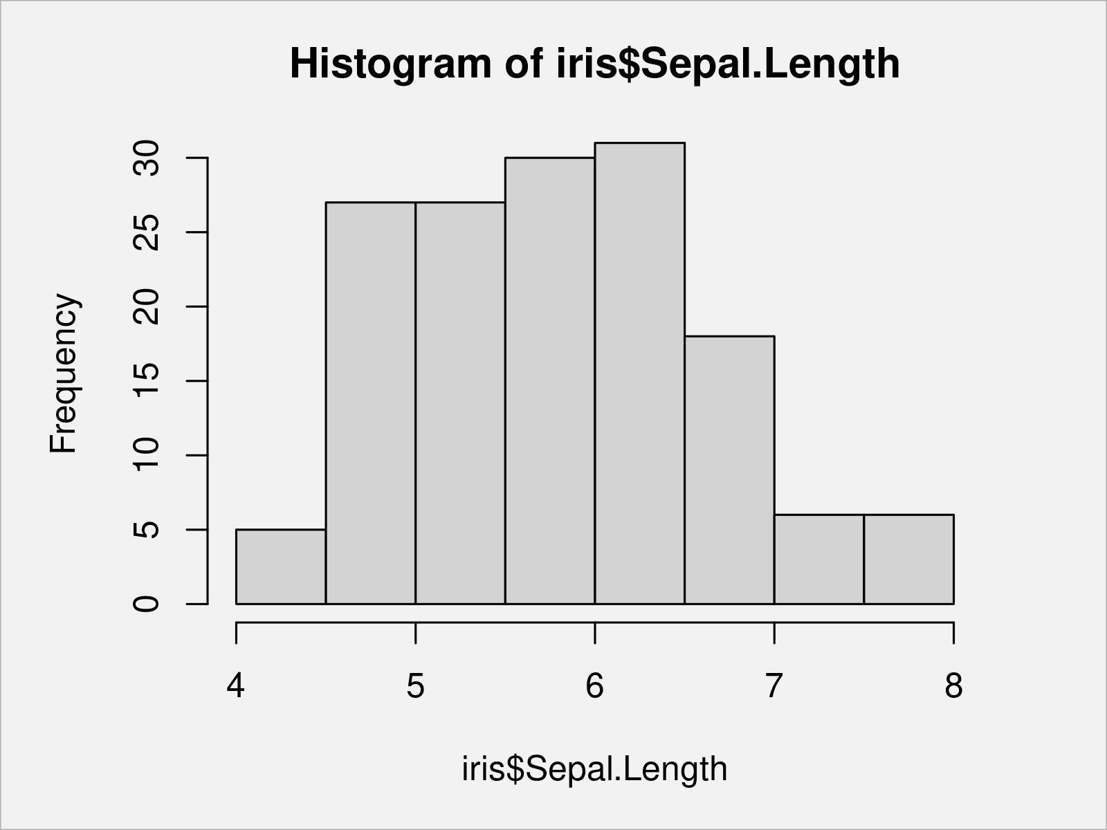
Similar to density plots, we can also draw a histogram of a certain vector object or a data frame column.

To accomplish this, we have to apply the hist function to one of the columns of our data frame:

hist(x = iris$Sepal.Length)                                               # Draw Base R histogram

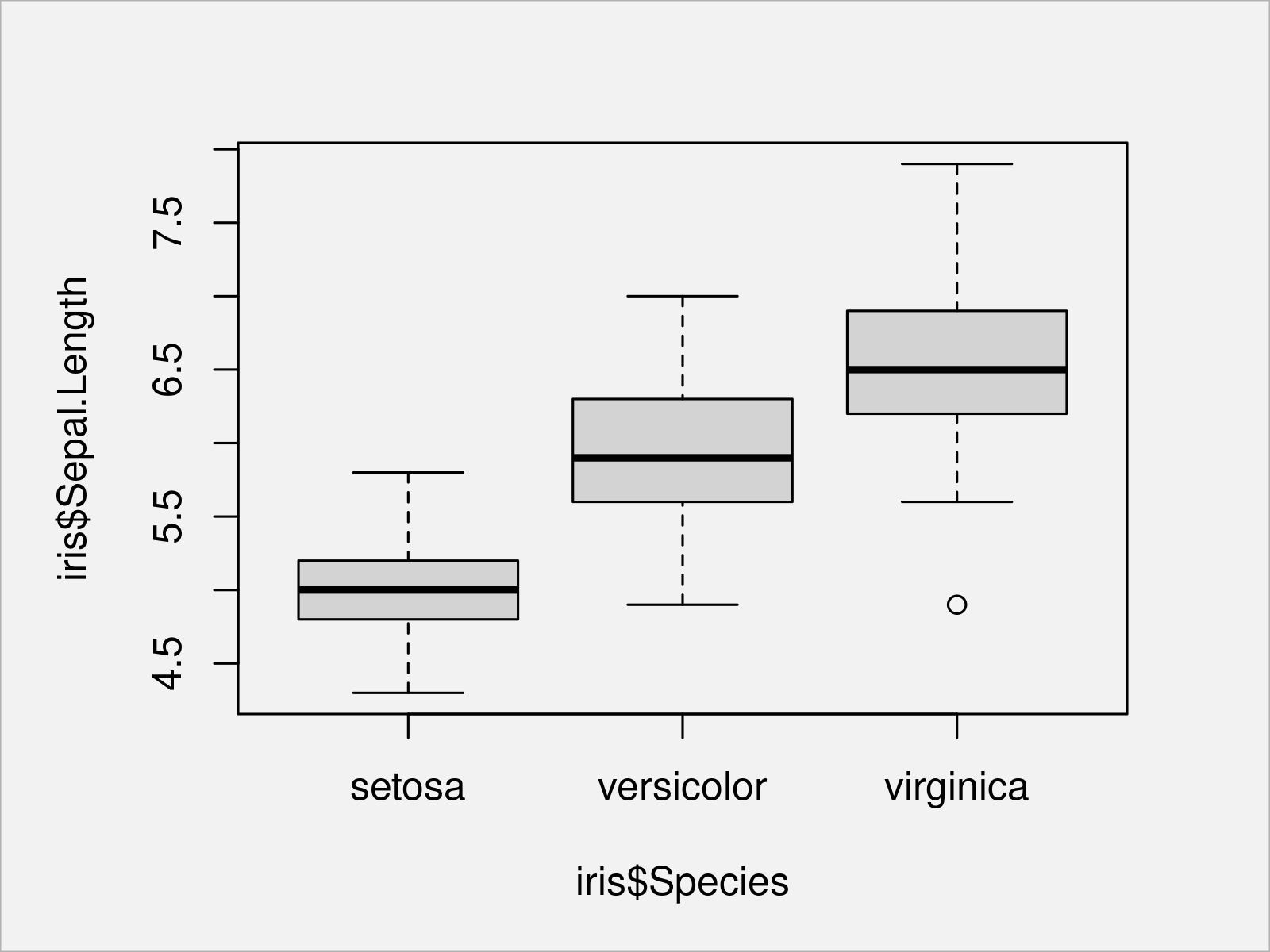
Another common kind of graph are so called boxplots (or box-and-whisker plots).

In the following example, we are creating a graphic containing multiple boxplots for the variable Sepal.Length side-by-side – One for each species in our data:

boxplot(iris$Sepal.Length ~ iris$Species)                                 # Draw Base R boxplot

As you have seen in the previous examples, the basic installation of the R programming language already provides many different ways to visualize your data; And I have only shown the tip of the iceberg here.

However, the R programming language provides a very powerful add-on package that provides even prettier solutions when creating graphics in R.

This package is called ggplot2, and in the following part of the tutorial I will focus on the creation of graphics using the ggplot2 package in R.

Let’s do this!

Creating Graphics Using the ggplot2 Package

To be able to use the functions of the ggplot2 add-on package, we first need to install and load ggplot2.

Generally speaking, the installation and loading of add-on packages is quite straightforward in the R programming language.

To accomplish this, we first have to install the package using the install.packages function. Note that this needs to be done only once on every computer:

install.packages("ggplot2")                                               # Install ggplot2 package

In the next step, we have to load the package using the library function. This needs to be done once per RStudio session:

library("ggplot2")                                                        # Load ggplot2

After executing the previous code, we can apply the functions of the ggplot2 package to draw different types of graphics.

When using the ggplot2 package, you have to know that the syntax for ggplot2 plots is typically structured into different parts:

1. The first part defines the data and variable names as well as the aesthetics of our plot (e.g. the colors). For this, we can use the ggplot and aes functions.
2. The second part specifies the kind of graph we want to create. Each type of graph can be created by a different geom_ function, e.g. density plots are created by the geom_density function.
3. The third part is optional and allows the user to modify certain components of a graphic. For instance, you may change the main and axis titles, or you may change the ordering and allocation of particular plot elements.

Note that the general guidelines above can vary depending on the plot you want to draw and depending on its complexity. However, especially for the basic plots these are good guidelines to keep in mind.

The first type of ggplot2 graph I want to show you is a scatterplot.

In the first part of the code below we specify that we want to use the iris data set as well as the Sepal.Length and Sepal.Width columns. Furthermore, we specify that we want to use a different color for each group in the Species column.

In the second part of the code we specify that we want to draw a scatterplot. For this, we can use the geom_point function.

Since we want to use the default settings for the other parameters of this plot, we don’t have to specify anything else.

Consider the R code below:

ggplot(iris,                                                              # Draw ggplot2 scatterplot
       aes(x = Sepal.Length,
           y = Sepal.Width,
           col = Species)) +
  geom_point()

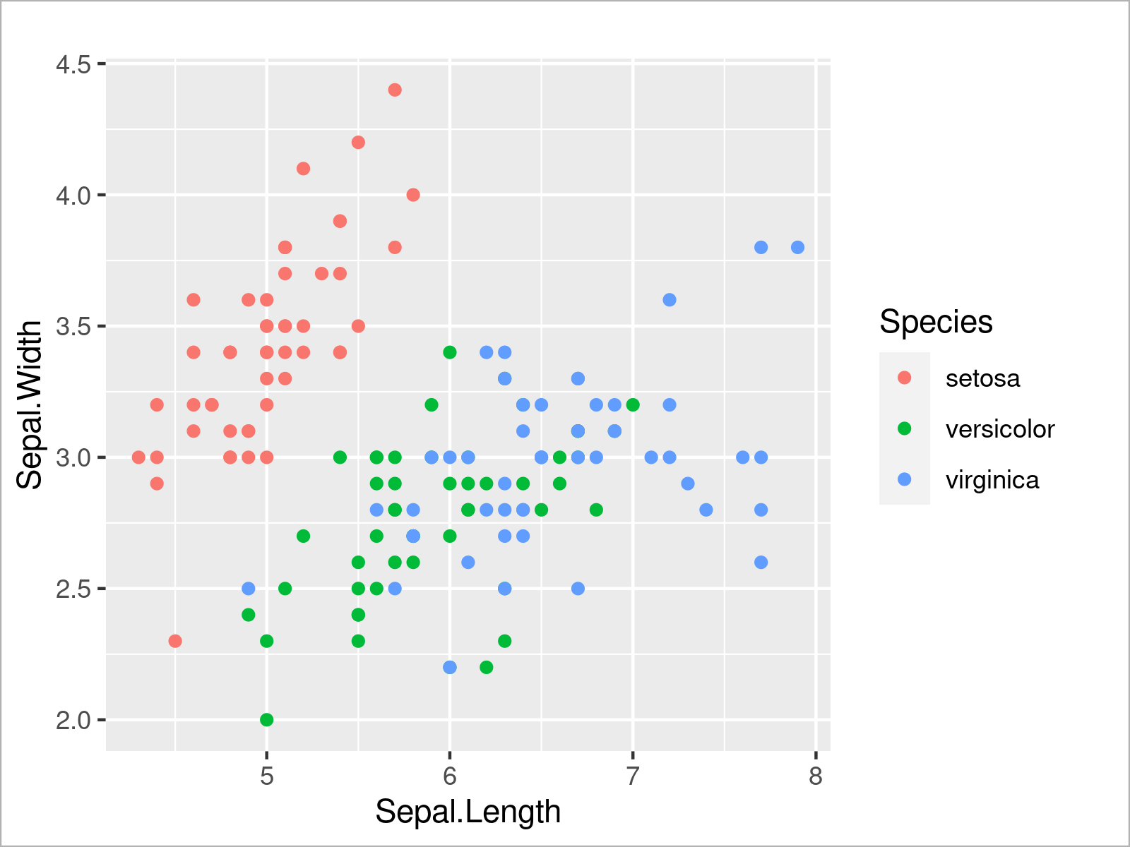
The output of the previous R code is shown in Figure 5 – We have created a ggplot2 scatterplot with different colors for each species.

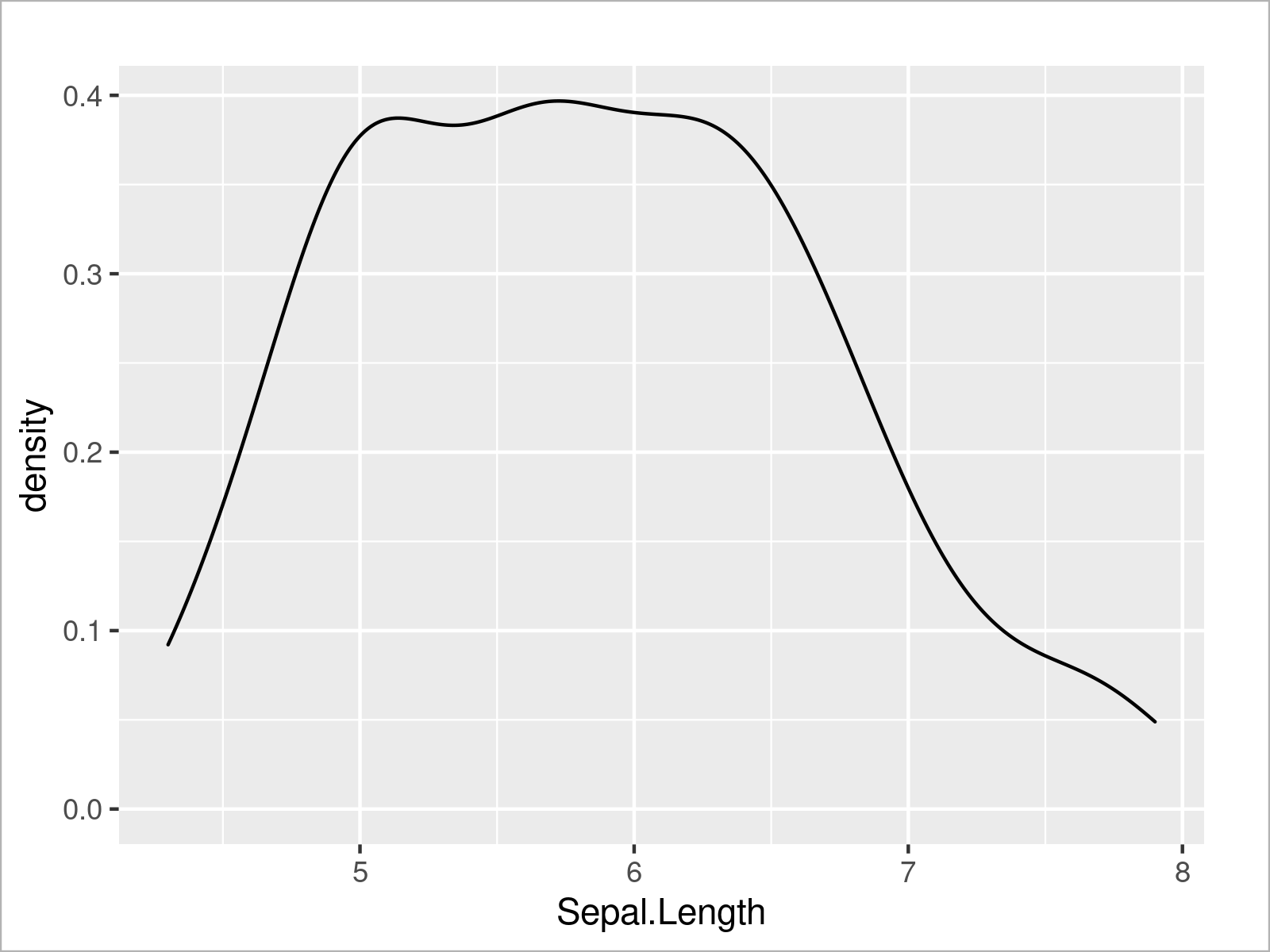
We can use a similar code to create other types of ggplot2 plots. The R code below demonstrates how to draw a ggplot2 density plot of the variable Sepal.Length:

ggplot(iris,                                                              # Draw ggplot2 density plot
       aes(x = Sepal.Length)) +
  geom_density()

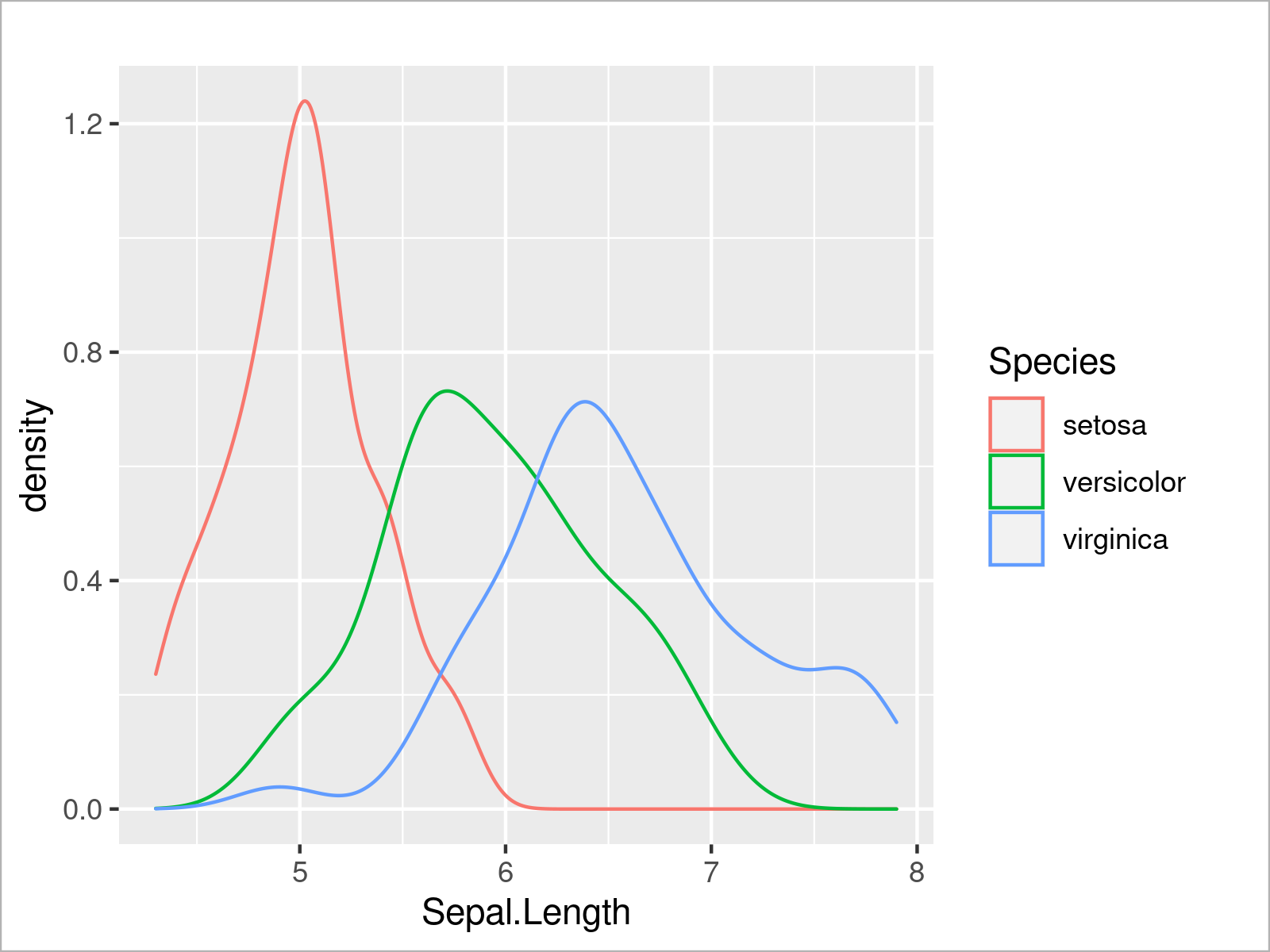
I very useful feature of the ggplot2 package is that we can create a graphic containing multiple plots within the same graphical window by simply specifying a certain grouping parameter within the aesthetics of the ggplot2 plot.

In the following code snippet, we set the color attribute within the aes function to be equal to the Species column of our data frame, and as visualized in the figure below, this creates a graphic with multiple overlaid density plots:

ggplot(iris,                                                              # Draw multiple ggplot2 density plots
       aes(x = Sepal.Length,
           col = Species)) +
  geom_density()

In addition to the color, we can also specify other arguments such as the filling color of each density:

ggplot(iris,                                                              # Fill ggplot2 density plots
       aes(x = Sepal.Length,
           col = Species,
           fill = Species)) +
  geom_density()

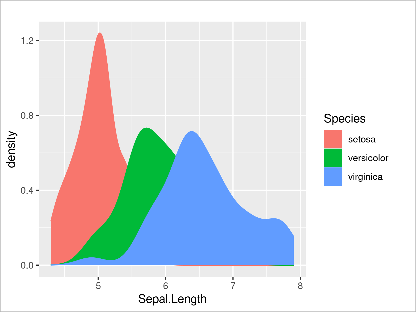
The output of the previous R syntax is shown in Figure 8: A ggplot2 graphic containing multiple densities with a filling color.

In the graph above some parts of some of the densities are completely overlaid by other densities. To avoid this problem, we can set the alpha argument within the geom_density function to a lower value to make our densities transparent:

ggplot(iris,                                                              # Opacity of ggplot2 density plots
       aes(x = Sepal.Length,
           col = Species,
           fill = Species)) +
  geom_density(alpha = 0.3)

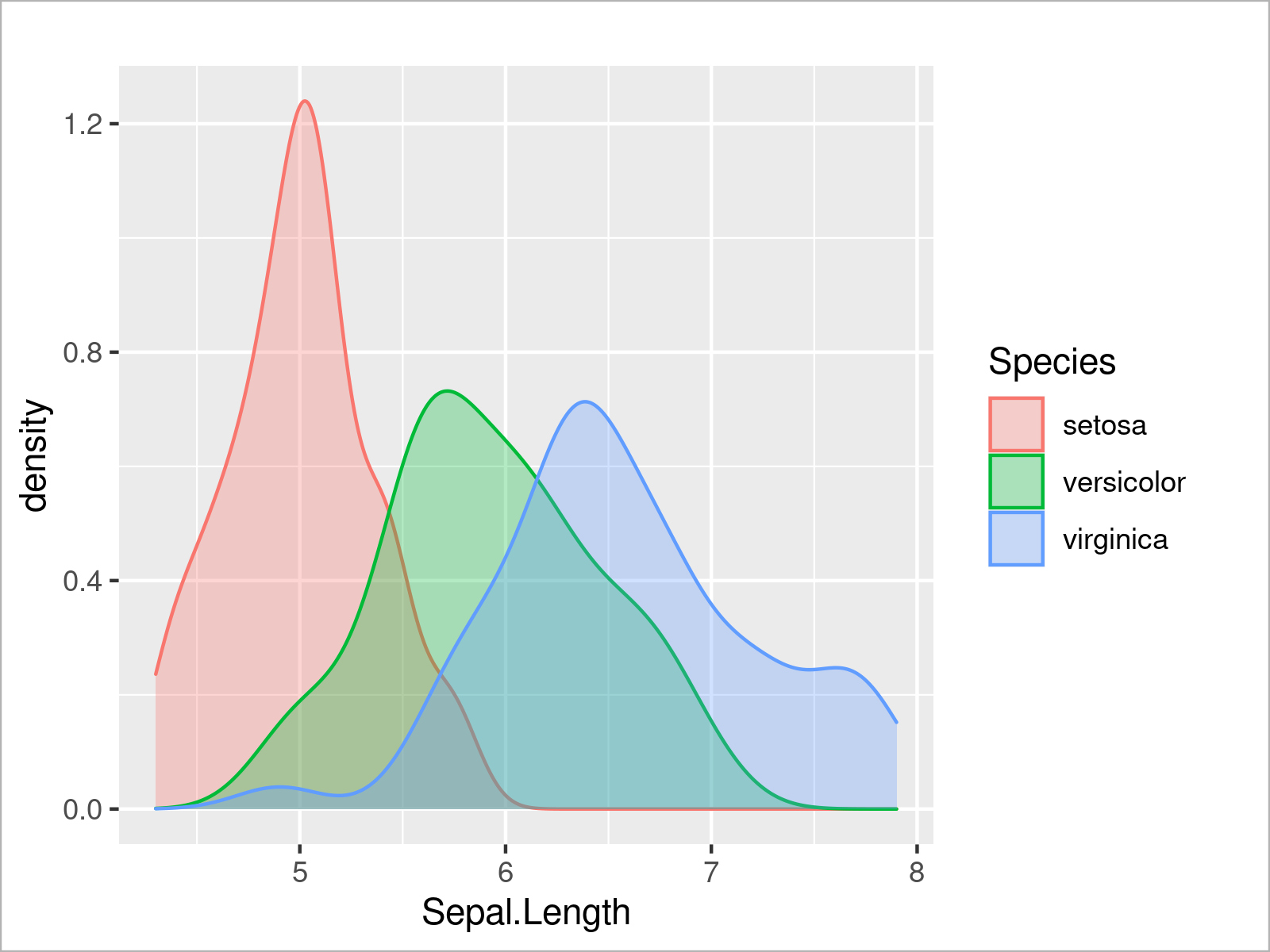
By running the previous R programming syntax, we have created Figure 9, i.e. a ggplot2 graph with multiple transparent densities.

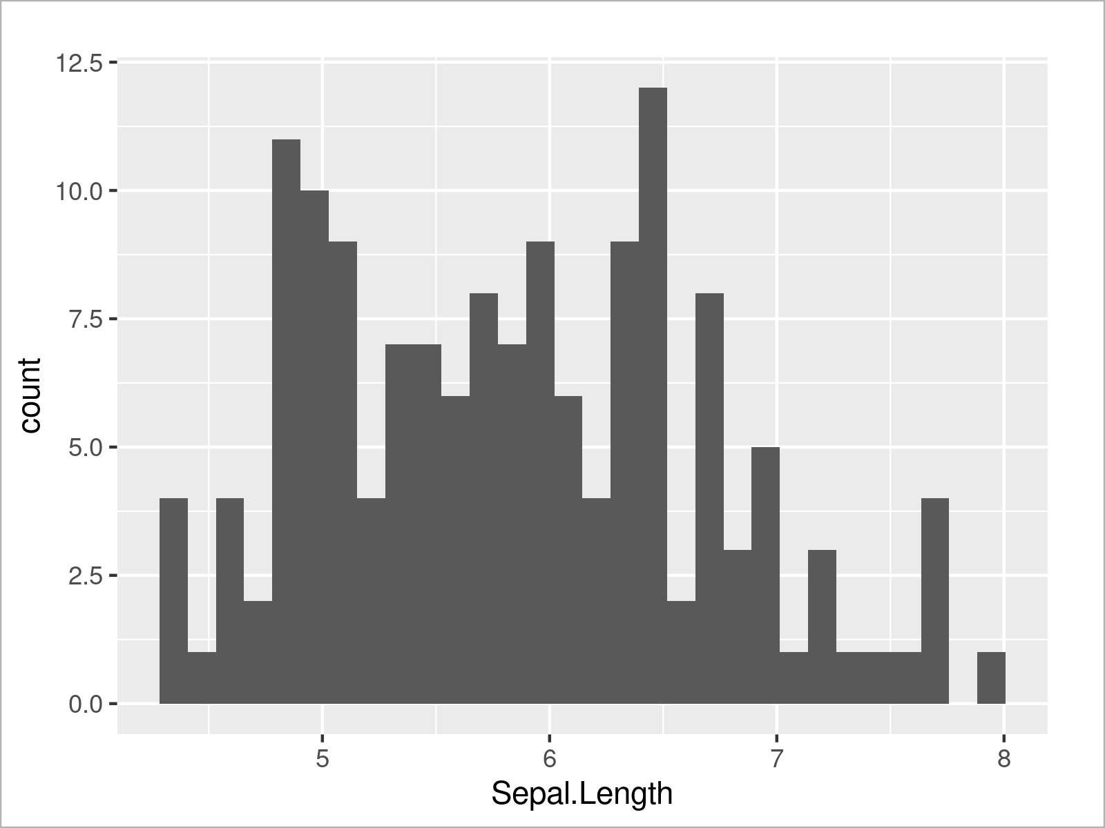
We can also use the ggplot2 package to create a histogram of a certain variable by using the geom_histogram function instead of the geom_density function:

ggplot(iris,                                                              # Draw ggplot2 histogram
       aes(x = Sepal.Length)) +
  geom_histogram()

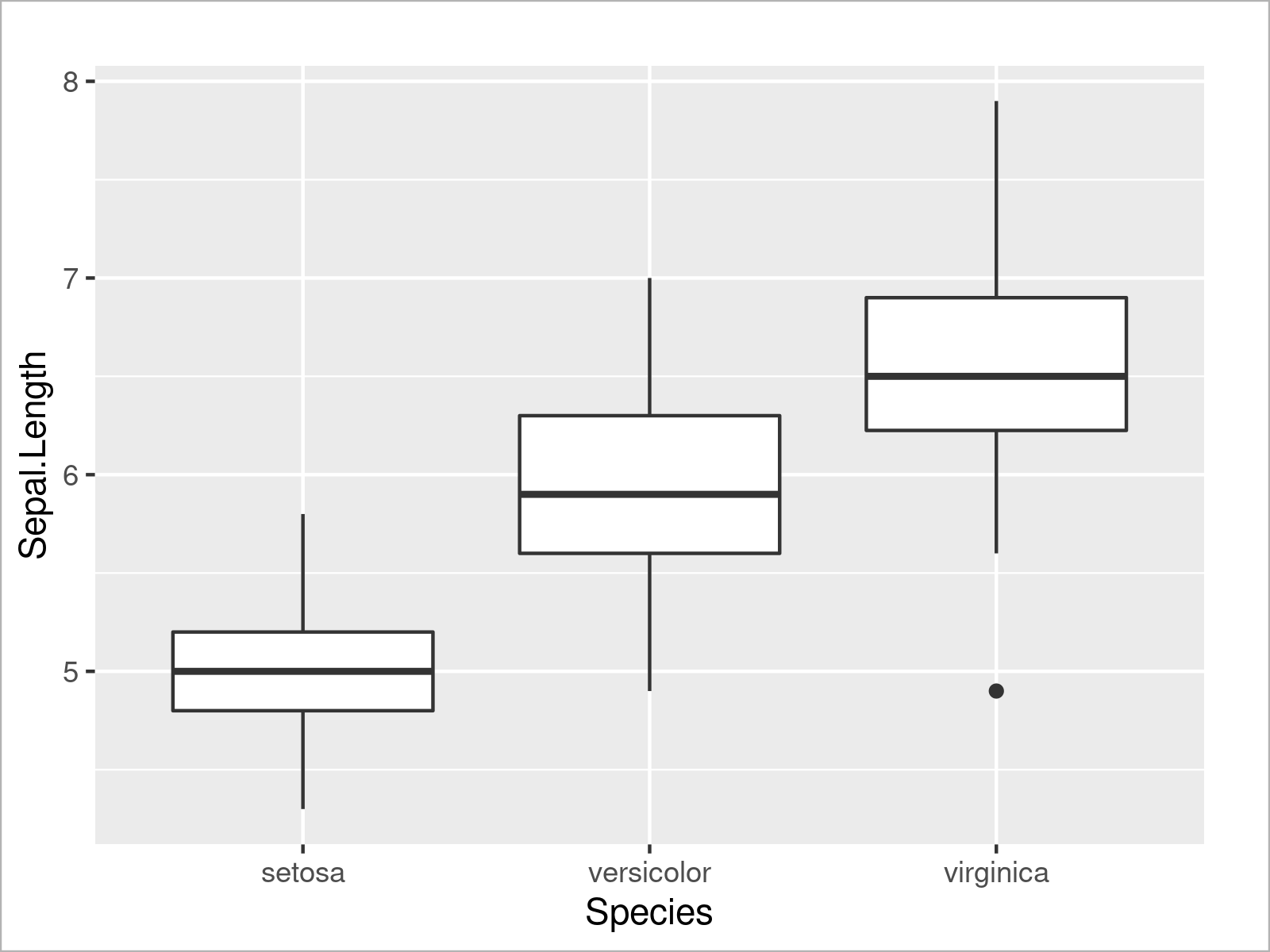
Furthermore, we can visualize our data in box-and-whisker plots:

ggplot(iris,                                                              # Draw ggplot2 boxplot
       aes(x = Species,
           y = Sepal.Length)) +
  geom_boxplot()

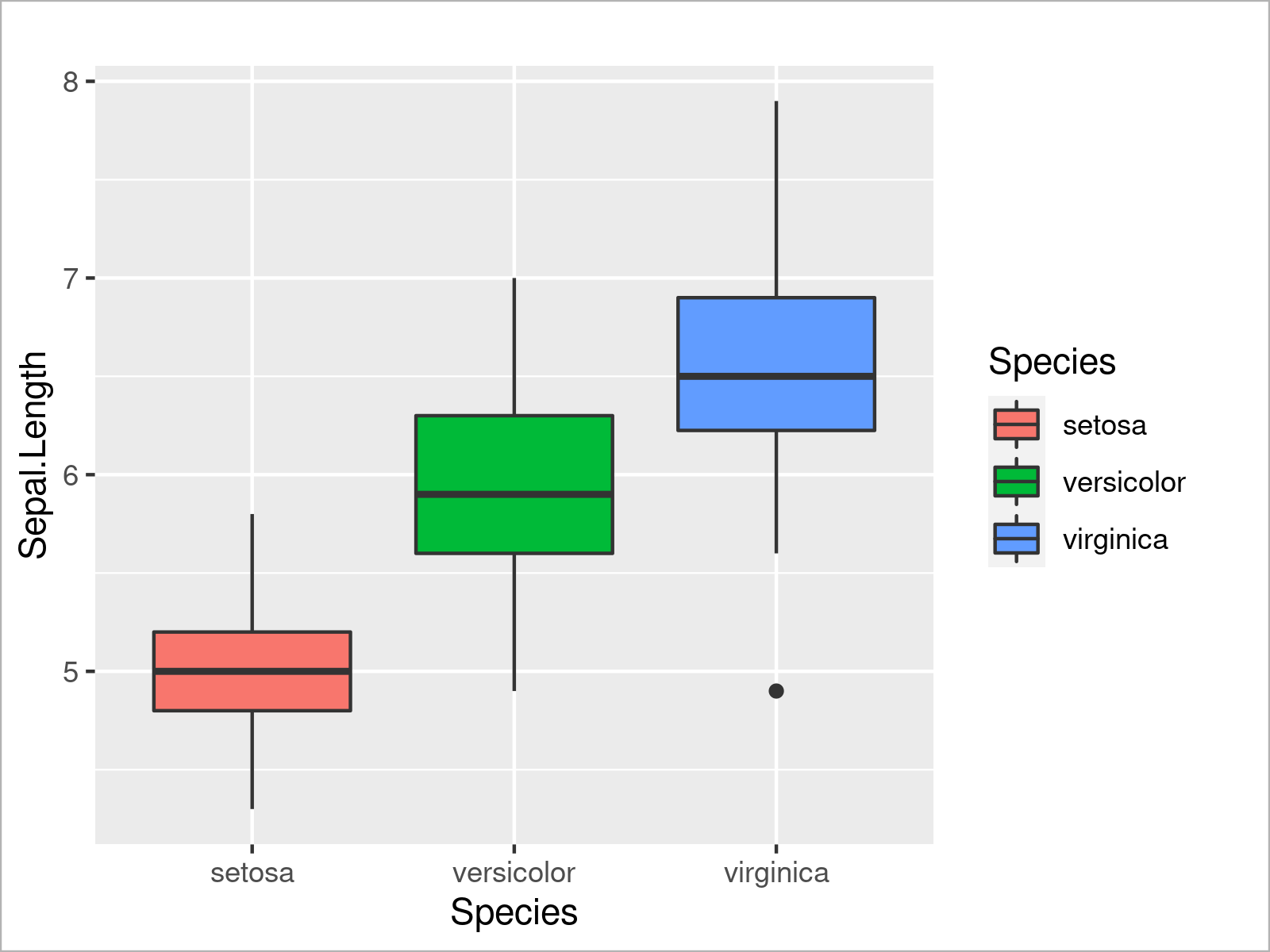
Similar to the example where we have drawn multiple densities, we can also draw multiple boxplots side-by-side by specifying a certain attribute within the aesthetics of the ggplot2 plot (i.e. the fill argument):

ggplot(iris,                                                              # Add colors to ggplot2 boxplot
       aes(x = Species,
           y = Sepal.Length,
           fill = Species)) +
  geom_boxplot()

As you have seen in the previous examples, the ggplot2 package is quite flexible and provides many different types of plots. However, there’s one very popular type of plot that we haven’t talked about yet: Barplots!

To draw a ggplot2 barplot, we first have to aggregate the values in our data:

iris_groups <- iris                                                       # Create duplicate of iris data set
iris_groups$Sub <- letters[1:3]                                           # Add subgroups to data
iris_groups <- aggregate(formula = Sepal.Length ~ Species + Sub,          # Mean by subgroup
                         data = iris_groups,
                         FUN = mean)
iris_groups                                                               # Print aggregated iris data set

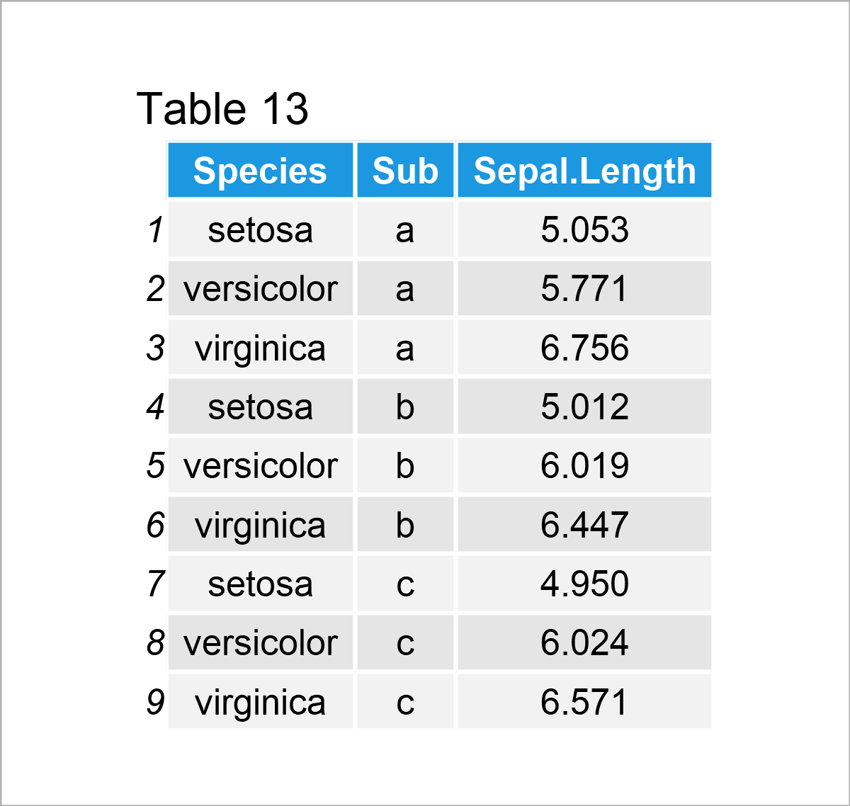
By executing the previous R syntax, we have created Table 13, i.e. a new data frame containing the mean value of the column Sepal.Length by each subgroup for each species.

We can now use this new data set to draw a ggplot2 barchart:

ggplot(iris_groups,                                                       # Draw ggplot2 barplot
       aes(x = Species,
           y = Sepal.Length)) +
  geom_bar(stat = "identity")

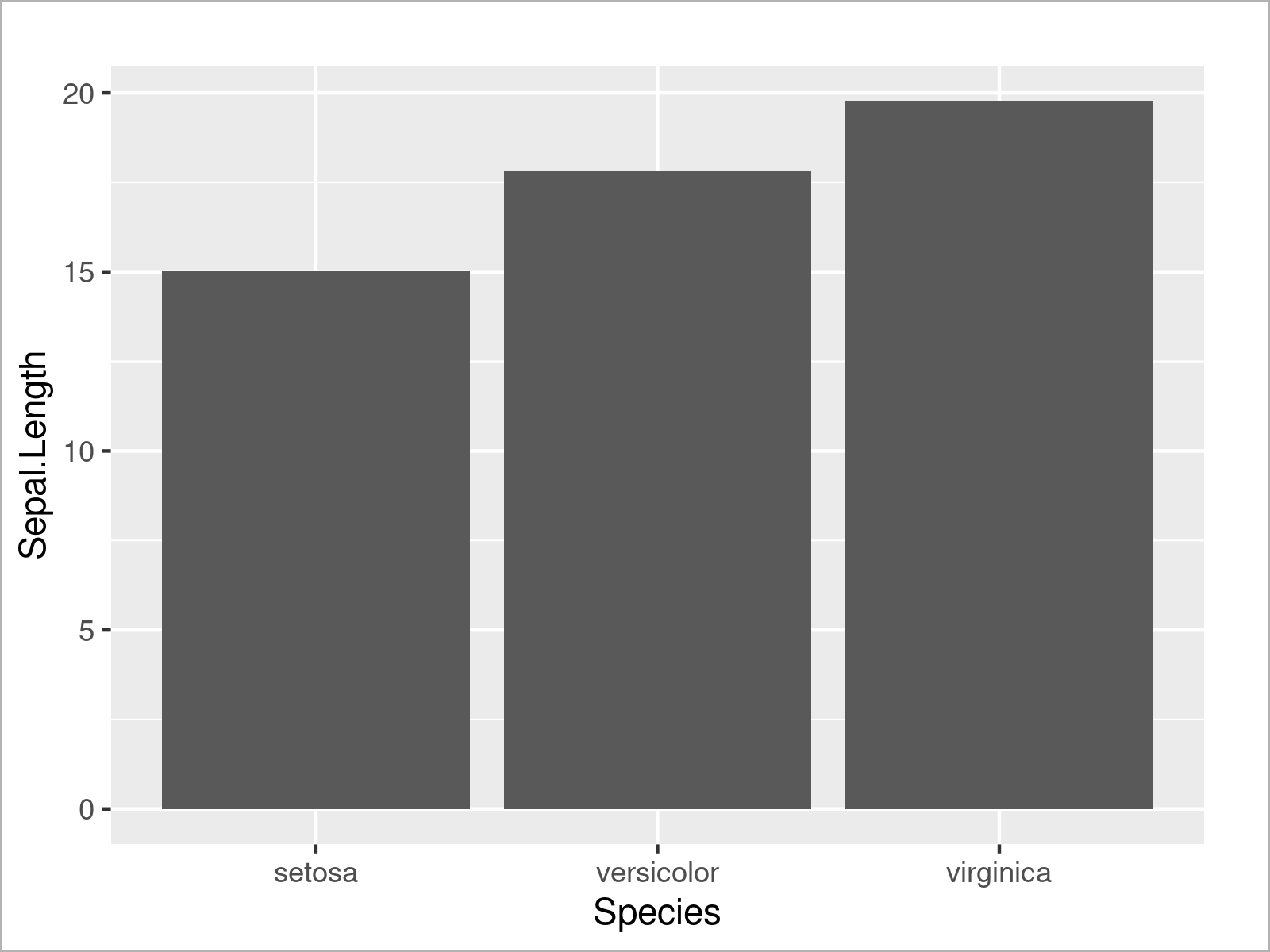
As shown in Figure 13, the previous R programming syntax has created a bargraph that contains one bar for the sum of all mean values of each species.

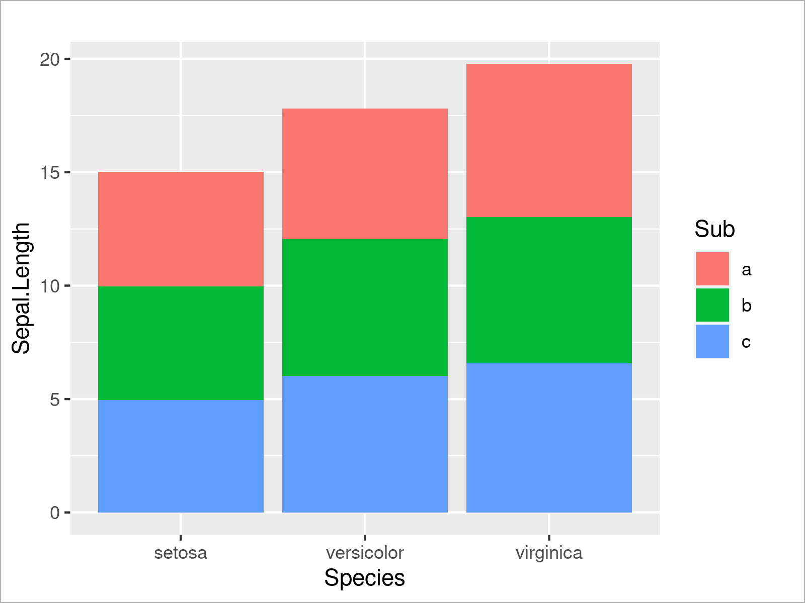
If we also want to take the subgroups into account, we can separate each of the bars in a so-called stacked barplot. For this, we have to set the fill argument to be equal to our subgroup column:

ggplot(iris_groups,                                                       # Draw stacked ggplot2 barplot
       aes(x = Species,
           y = Sepal.Length,
           fill = Sub)) +
  geom_bar(stat = "identity")

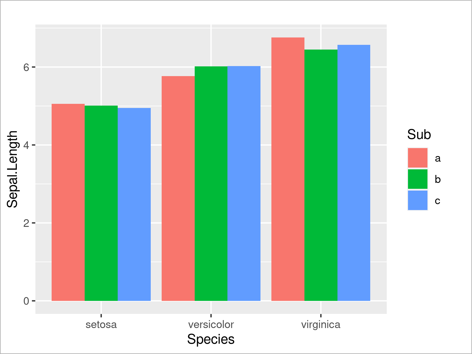
Alternatively to this, we can also separate the subgroups in each species by drawing a grouped barchart. To complete this, we have to set the position argument within the geom_bar function to “dodge”:

ggplot(iris_groups,                                                       # Draw grouped ggplot2 barplot
       aes(x = Species,
           y = Sepal.Length,
           fill = Sub)) +
  geom_bar(stat = "identity",
           position = "dodge")

This section has demonstrated the strength of R when it comes to the visualization of data in different kinds of graphics.

Note that this section has only illustrated some of the most popular ways to visualize data in R. However, the R programming language provides basically unlimited ways to draw your data!

Have a look at this tutorial for more details.

Graphical visualization is only one approach when analyzing data. In the next section I’ll show some techniques to analyze your data based on descriptive metrics and statistical models.

Let’s dive into it!

Data Analysis & Descriptive Statistics in R

This section demonstrates different methods on how to analyze data in the R programming language.

We’ll start with some basic metrics, and then we’ll move on to some more advanced statistical models.

So without too much talk, let’s do this!

Calculate Basic Statistical Metrics

In the following part of the tutorial, I’ll show how to calculate basic descriptive statistics in R.

We’ll use the vector object vec_1 that we have created at the beginning of this tutorial as a basis. However, please note that we could apply the following R syntax to data frame columns or to more complex data as well.

The R programming language provides functions for basically all important statistical metrics.

For instance, we can calculate the mean of a vector object by using the mean function:

mean(vec_1)                                             # Calculate mean
# [1] 2.666667

As you can see based on the previous output of the RStudio console, the mean of our vector object is 2.666667.

Similar to this, we can apply other functions to our vector object to compute other summary statistics.

For instance, we can calculate the median using the median function…

median(vec_1)                                           # Calculate median
# [1] 2

…the minimum value using the min function…

min(vec_1)                                              # Calculate minimum
# [1] 1

…the maximum value by applying the max function…

max(vec_1)                                              # Calculate maximum
# [1] 5

…the sum using the sum function…

sum(vec_1)                                              # Calculate sum
# [1] 16

…the variance by applying the var function…

var(vec_1)                                              # Calculate variance
# [1] 3.866667

and the standard deviation by using the sd function:

sd(vec_1)                                               # Calculate standard deviation
# [1] 1.966384

If we want to calculate multiple summary statistics with a single function call, we can apply the summary function as shown below.

As you can see, the summary function returns the minimum, first quartile, median, mean, third quartile, and the maximum value of a data object:

summary(vec_1)                                          # Calculate multiple descriptive statistics
#  Min. 1st Qu.  Median    Mean 3rd Qu.    Max. 
# 1.000   1.000   2.000   2.667   4.500   5.000

In case we want to get the frequency counts of certain values in a data object, we can apply the table function.

The R code below demonstrates how to calculate a frequency table. As you can see, the value 1 appears three times in our vector, the value 3 occurs only once, and the value 5 is appearing twice:

table(vec_1)                                            # Create frequency table
# vec_1
# 1 3 5 
# 3 1 2

We can also use the table function to get a contingency table across two or multiple columns.

The following R code prints the contingencies for the combinations of two data frame columns x1 and x2 of our data frame data_1 that we have created in the data manipulation section.

For example, the combination of the value 2 in the variable x1 with the value x in the variable x2 appears 0 times (i.e. not at all). The combination of the value 3 in the variable x1 with the value x in the variable x3 occurrs twice:

table(data_1[ , c("x1", "x2")])                         # Create contingency table
#    x2
# x1  x y
#   2 0 1
#   3 2 0
#   7 1 1
#   8 1 0

The previous R code has demonstrated how to measure simple descriptive statistics.

However, the R programming language can also be used to estimate more complex statistical models, and this is what we will do in the next section!

Estimation of Regression Models

In the following part, we’ll use once again the iris data set that we have already loaded in the data visualization section.

Probably the most common statistical model is the so-called linear regression model.

We can estimate such a regression model with Sepal.Width as dependent variable (or outcome; target variable) and the variable Sepal.Length as independent variable (or predictor) using the lm function as shown below:

mod_1 <- lm(formula = Sepal.Width ~ Sepal.Length,       # Estimate linear regression model
            data = iris)

The previous R syntax has created a new model object called mod_1. We can now use the summary function to print certain summary statistics for this model to the RStudio console:

summary(mod_1)                                          # Summary statistics of model
# Call:
# lm(formula = Sepal.Width ~ Sepal.Length, data = iris)
# 
# Residuals:
#     Min      1Q  Median      3Q     Max 
# -1.1095 -0.2454 -0.0167  0.2763  1.3338 
# 
# Coefficients:
#              Estimate Std. Error t value Pr(>|t|)    
# (Intercept)   3.41895    0.25356   13.48   <2e-16 ***
# Sepal.Length -0.06188    0.04297   -1.44    0.152    
# ---
# Signif. codes:  0 ‘***’ 0.001 ‘**’ 0.01 ‘*’ 0.05 ‘.’ 0.1 ‘ ’ 1
# 
# Residual standard error: 0.4343 on 148 degrees of freedom
# Multiple R-squared:  0.01382,	Adjusted R-squared:  0.007159 
# F-statistic: 2.074 on 1 and 148 DF,  p-value: 0.1519

As you can see, the previous output is relatively complex. Besides many other things, it shows certain metrics for the residuals of our model, the regression coefficients with significance stars, the residual standard error, the multiple and adjusted R-squared, the F-statistic, the degrees of freedom, and the p-value.

The explanation for all of these metrics would go beyond the scope of this tutorial. However, I recommend having a look here for a detailed instruction on how to interpret the output of regression models.

What is particularly interesting about the model output is that the regression coefficient for the variable Sepal.Length is not significant.

This might be surprising, since one might guess that the length of a petal would be somehow related to the petal width.

Let’s use our data visualization skills that we have gathered in the previous section to visualize our data once again:

ggplot(iris,                                            # Draw scatterplot with regression line
       aes(x = Sepal.Length,
           y = Sepal.Width)) +
  geom_point() +
  geom_smooth(method = "lm")

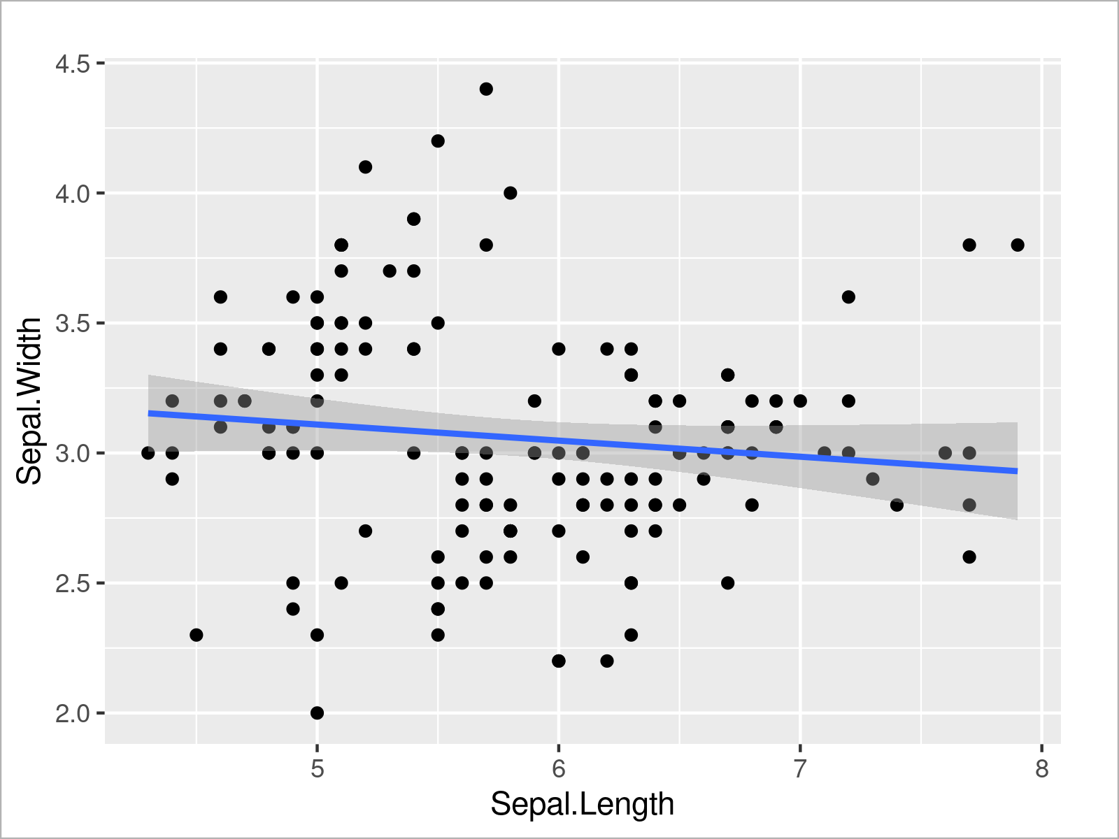
The previous R code has created a scatterplot with a regression line on top.

As you can see, the regression slope is relatively flat, which seems to confirm the non-significant result of our linear regression model.

However, in the graphic we can also see that there seem to be different clusters (i.e. the species groups) in our data. For that reason, it might make sense to add another predictor variable to our model.

The following R code estimates a multivariate linear regression model using the variables Sepal.Length and Species as predictors for the target variable Sepal.Width:

mod_2 <- lm(formula = Sepal.Width ~ Sepal.Length + Species, # Model with multiple predictors
            data = iris)

Next, we can return the summary of this model:

summary(mod_2)                                          # Summary statistics of model
# Call:
# lm(formula = Sepal.Width ~ Sepal.Length + Species, data = iris)
# 
# Residuals:
#      Min       1Q   Median       3Q      Max 
# -0.95096 -0.16522  0.00171  0.18416  0.72918 
# 
# Coefficients:
#                   Estimate Std. Error t value Pr(>|t|)    
# (Intercept)        1.67650    0.23536   7.123 4.46e-11 ***
# Sepal.Length       0.34988    0.04630   7.557 4.19e-12 ***
# Speciesversicolor -0.98339    0.07207 -13.644  < 2e-16 ***
# Speciesvirginica  -1.00751    0.09331 -10.798  < 2e-16 ***
# ---
# Signif. codes:  0 ‘***’ 0.001 ‘**’ 0.01 ‘*’ 0.05 ‘.’ 0.1 ‘ ’ 1
# 
# Residual standard error: 0.289 on 146 degrees of freedom
# Multiple R-squared:  0.5693,	Adjusted R-squared:  0.5604 
# F-statistic: 64.32 on 3 and 146 DF,  p-value: < 2.2e-16

As you can see, our multivariate model shows many different regression coefficients, and all of these coefficients are significant. Even the variable Sepal.Length that was measured to be not significant in the previous model is now highly significant.

The reason for this is that the variable Species is a confounder that has ruined the measurement of the relation between Sepal.Width and Sepal.Length in the first model.

We can illustrate the relations between the variables Sepal.Length and Sepal.Width within each species group by drawing a ggplot2 plot with a separate regression line for each group.

Note that the following plot does not show the same regression slop as our previously estimated model. However, we can use it to visualize the differences by group.

However, the following plot shows that all the three regression lines do clearly have a positive slope.

ggplot(iris,                                            # Draw multiple regression lines
       aes(x = Sepal.Length,
           y = Sepal.Width,
           col = Species)) +
  geom_point() +
  geom_smooth(method = "lm")

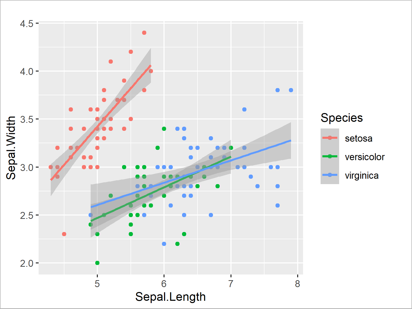
In this section, you have learned how to analyze your data using basic statistical metrics as well as statistical regression models.

Note that the methods shown in this section are still very basic, and that the R programming language provides much more advanced modelling techniques.

You may have a look here for some further reading on this topic.

At this point, I want to move on to the last section of the present tutorial. In this section I will demonstrate some more advanced programming techniques to give you an idea of what is possible with the R programming language once you become a more advanced R programmer.

Advanced Techniques in R

This section demonstrates some more advanced programming techniques in the R programming language.

I’ll first explain how to use loops, then we’ll move on to if else statements, and last but not least you’ll learn how to create your own functions.

Loop Over Vectors & Data Frame Rows

Loops are an often used technique in most programming languages.

In this section, I’ll demonstrate how to loop over the elements of a vector object, and over the rows of a data frame.

We’ll start off by creating an empty numeric vector object of zero length:

vec_6 <- numeric()                                      # Create empty numeric vector
vec_6                                                   # Print empty numeric vector
# numeric(0)

This vector will be used to store the outputs of the following loop.

Loops in R can typically be divided into two different parts:

• The head of the loop defines a running index and the elements through which the loop should be iterated.
• The body of the loop defines what kind of operation should be applied within each iteration of the loop.

In the next lines of code, I’m applying a for-loop to the elements of our vector object vec_1.

In the body of the loop I’m specifying that I want to calculate the sum of the ith element of the loop and the running index i. This output should then be stored at the ith position of the empty vector object vec_6.

for(i in 1:length(vec_1)) {                             # Apply for loop to vector
  vec_6[i] <- vec_1[i] + i
}

Our previously empty vector object vec_6 is updated after running the previous for-loop. Let’s first have a look at our input vector vec_1:

vec_1                                                   # Print vec_1 for comparison
# [1] 1 1 5 3 1 5

And then let’s have a look at the output vector vec_6:

vec_6                                                   # Print new vector
# [1]  2  3  8  7  6 11

As you can see, the output vector vec_6 contains six new elements. Those elements have been calculated within the for-loop as shown below:

• Iteration 1) 1 + 1 = 2
• Iteration 2) 1 + 2 = 3
• Iteration 3) 5 + 3 = 8
• Iteration 4) 3 + 4 = 7
• Iteration 5) 1 + 5 = 6
• Iteration 6) 5 + 6 = 11

In the previous example we have looped through the elements of a vector. However, we can use a similar syntax to loop over the rows of a data frame.

For this, we first have to construct a data frame through which we want to loop:

data_12 <- data_1                                       # Create duplicate of data frame
data_12$x4 <- NA                                        # Add new column containing only NA
data_12                                                 # Print new data frame

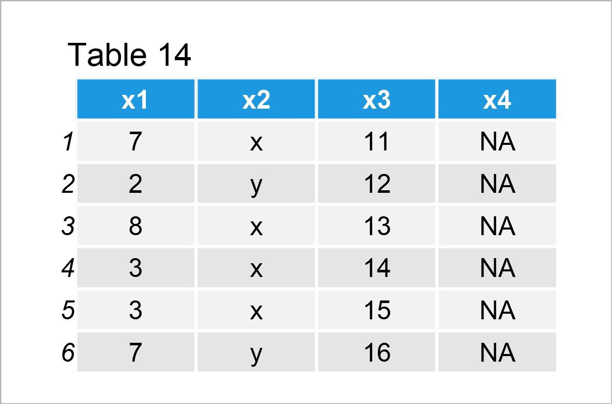
As you can see in the previous table, we have created a data frame called data_12 containing the three columns of our data frame data_1 plus a fourth column that contains only NA values.

We can now use a for-loop to iterate over the rows of this data frame, and to store new values in the empty column based on this loop:

for(i in 1:nrow(data_1)) {                              # Loop over rows of data frame
  data_12$x4[i] <- data_12$x1[i] + i * data_12$x3[i]
}

Let’s have another look at our data frame data_12:

data_12                                                 # Print updated data frame

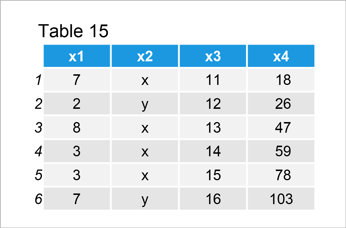
The previous table shows that we have filled up the NA elements of the variable x4 with new values. Looks good!

In the previous examples we have used for-loops to iterate through vector elements and data frame rows. Note that the R programming language also provides other types of loops such as while-loops and repeat-loops.

Furthermore, please note that loops in R are a very controversial topic. Many people argue that loops are slow and not the best programming practice. Hence, they prefer to avoid for-loops at all.

In my personal opinion, loops are often more intuitive than their alternatives and, for that reason, I use loops when I’m dealing with smaller data sets where speed does not matter too much. When I’m dealing with larger data sets, I also prefer to use more efficient techniques such as the Family of apply functions.

In case you want to read more about this loop-discussion, you may have a look at this article.

However, let’s move on to the next advanced programming technique – if else statements!

If Else Statements

If else statements – as indicated by the name – are usually used to create two different outputs depending on a logical condition.

If this condition is true, output A should be returned; If this condition is false, output B should be returned.

The following R code shows how to use such an if else statement within a for-loop.

For this example, we first have to create an empty character vector:

vec_7 <- character()                                    # Create empty character vector
vec_7                                                   # Print empty character vector
# character(0)

Next, we can run a for-loop over the elements in our vector object vec_1, and within this loop we can apply an if else statement to create a binary output.

In case the logical condition vec_1[i] > 3 is TRUE, the character string “high” should be assigned to the empty vector vec_7; and in case the logical condition vec_1[i] > 3 is FALSE, the character string “low” should be assigned to the empty vector vec_7.

for(i in 1:length(vec_1)) {                             # for loop & nested if else statement
  if(vec_1[i] > 3) {
    vec_7[i] <- "high"
  } else {
    vec_7[i] <- "low"
  }
}

Let’s print the vector vec_7 once again:

vec_7                                                   # Print updated vector
# [1] "low"  "low"  "high" "low"  "low"  "high"

As you can see, we have assigned the character strings “high” and “low” to this vector, depending on the logical condition in the if statement.

This worked fine, but the previous code was kind of complicated. Fortunately, the R programming language provides a convenient alternative – the ifelse function.

Within the ifelse function, we have to specify three arguments:

• The logical test condition.
• The output in case of this condition is TRUE.
• The output in case of this condition is FALSE.

Consider the following example code:

vec_8 <- ifelse(test = vec_1 > 3,                       # Apply ifelse function
                yes = "high",
                no = "low")

After executing the previous R code, the new vector object vec_8 has been created:

vec_8                                                   # Print new vector
# [1] "low"  "low"  "high" "low"  "low"  "high"

As you can see, this vector object contains exactly the same elements as the output vector vec_7 that we have created with the previous for-loop and if else statement. However, this time the code was much simpler.

User-Defined Functions

Another very useful programming technique is the creation of user-defined functions.

Always when you have to run a certain type of code multiple times, you might save this code in your own function and run this function instead of the entire code.

This can help to shorten your code tremendously, and to make your code more efficient.

The R syntax below shows a simple example on how to create a user-defined function in R.

In this code, we define a new function called fun_1. This function takes an input value x, and in the body of this function some calculations are performed based on x. At the end of the function, the result of this calculation is returned.

Let’s create the function:

fun_1 <- function(x) {                                  # Create simple user-defined function
  out <- x^2 + 5 * x
  out
}

After running the syntax above, we can apply the function fun_1 as we would apply any other pre-defined function.

For instance, we can apply our function to the elements in the vector object vec_1:

fun_1(x = vec_1)                                        # Apply simple user-defined function
# [1]  6  6 50 24  6 50

The previous R code has shown an elementary user-defined function. However, you can make your functions as complex as you want.

The following R code shows how to create a user-defined function containing an if else statement:

fun_2 <- function(x, y) {                               # Create complex user-defined function
  if(y > 3) {
    out <- (x^2 + 5 * x) / y
  } else {
    out <- (x^2 + 5 * x) / (10 * y)
  }
  out
}

Now, we may apply this user-defined function within a for-loop:

for(i in 1:5) {                                         # Complex user-defined function in for loop
  print(paste0("This is the result of iteration ",
              i,
              ": ",
              fun_2(x = 5, y = i)))
}
# [1] "This is the result of iteration 1: 5"
# [1] "This is the result of iteration 2: 2.5"
# [1] "This is the result of iteration 3: 1.66666666666667"
# [1] "This is the result of iteration 4: 12.5"
# [1] "This is the result of iteration 5: 10"

As you can see, the previous R code has returned a result of our function for each iteration of the for-loop.

In this tutorial, I have demonstrated some of the most important statistical methods and programming techniques provided by the R programming language.

However, the R programming language provides much more than what I have shown on this page!

In case you are interested to learn more about R, you may check out the list of tutorials below.

It shows all R programming tutorials on Statistics Globe, and I’m providing instructions on a wide range of topics.

Furthermore, you might use the search button at the top right in the menu bar to navigate through the R programming tutorials on this website.

Let me know in the comments in case you have any further questions or recommendations.

I wish you a lot of success and endurance while learning R – it’s definitely worth it! 🙂

All R Programming Tutorials on Statistics Globe

You can find a list of all R tutorials on statisticsglobe.com below. In the tutorials, I’m explaining statistical concepts and provide reproducible example codes for beginners and advanced users in R.

3D Plot of PCA in R (2 Examples)

3D plotly Graph in R (3 Examples)

abline Function in R (6 Examples)

Access & Collect Data with APIs in R (Example)

Access & Manipulate Body of Function in R (2 Examples) | body() Command

Access Attributes of Data Object in R (2 Examples)

Access Index Names of List Using lapply Function in R (Example)

Add & Remove Trace in plotly Graph in R (3 Examples)

Add & Subtract Days to & from Date in R (2 Examples)

Add & Subtract Months & Years to/from Date Object in R (2 Examples)

Add Arrow to Plot in R (2 Examples)

Add Axes to Plot Using axis Function in R (4 Examples)

Add Bold & Italic Text to ggplot2 Plot in R (4 Examples)

Add Characters to Numeric Data Frame Column in R (2 Examples)

Add Color Between Two Points of Kernel Density Plot in R (Example)

Add Color to Region Between Two Lines in ggplot2 Line Plot in R (2 Examples)

Add Common Legend to Combined ggplot2 Plots in R (Example)

Add Confidence Band to ggplot2 Plot in R (Example)

Load More