Data Manipulation in R (9 Examples)

This article shows how to manipulate data frames in R programming.

Table of contents:

You’re here for the answer, so let’s get straight to the exemplifying R code!

Creation of Example Data

To begin with, we need to load some exemplifying data. In this tutorial, we’ll use the iris flower data set. We can load this data set using the data() function as shown below:

data(iris)                                            # Load iris data set

We can now use the head() function to print the first six rows of the iris data set to the RStudio console:

head(iris)                                            # Print first six rows of data frame

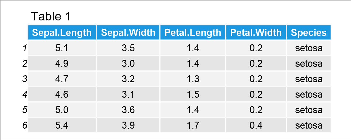
Table 1 shows the first six rows of our example data.

The variables Sepal.Length, Sepal.Width, Petal.Length, and Petal.Width are numerical, and the variable Species has the factor class.

As indicated by the column names, the rows of this data set contain information on different flowers, i.e. the length and width of certain components and the flower species.

In the following examples, I’ll use this data set to demonstrate some of the most important techniques for the wrangling and manipulation of data frames in R.

Let’s do this!

Example 1: Select Column of Data Frame

In Example 1, I’ll demonstrate how to extract a certain column from a data frame.

For this task, we can use the $ operator as shown in the following R code:

my_col <- iris$Sepal.Length                           # Convert column to vector

The previous R code has created a new data object called my_col. This data object contains the values of the column Sepal.Length.

We can print the first six elements of this data object using the head function:

head(my_col)                                          # First six elements of vector
# [1] 5.1 4.9 4.7 4.6 5.0 5.4

We might now analyze this data object as desired. Just to show you an example, the following R code calculates the mean value of our data object:

mean(my_col)                                          # Calculate mean of vector
# [1] 5.843333

Example 2: Remove Column from Data Frame

Example 2 shows how to delete particular columns from a data frame.

For this example, I’m first creating a duplicate of our example data frame, since I want to keep an original version of the example data:

irisA <- iris                                         # Duplicate data frame

After running the previous lines of code, a new data frame object called irisA has been created, which contains exactly the same values as the original iris data frame.

Next, we can use the colnames function and the != operator to drop a specific column (i.e. the variable Sepal.Length):

irisA <- irisA[ , colnames(irisA) != "Sepal.Length"]  # Drop one column
head(irisA)                                           # Print first six rows of data frame

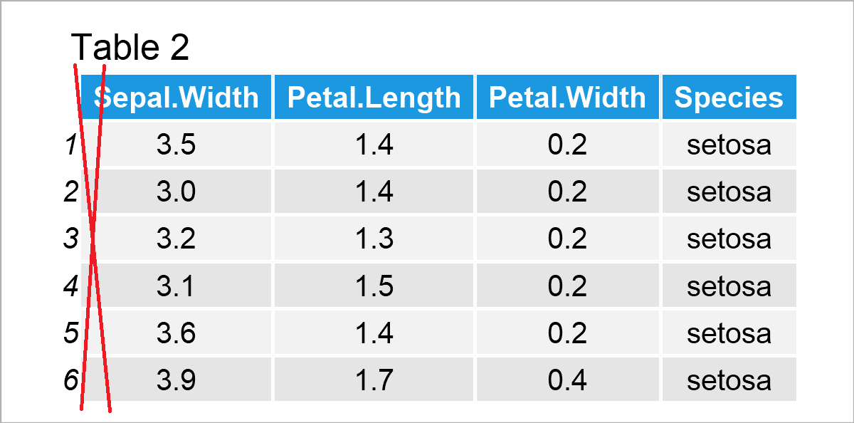
After executing the previous R programming syntax the new data frame shown in Table 2 has been created. As you can see, we have removed the column Sepal.Length.

Example 3: Add New Column to Data Frame

In this example, I’ll demonstrate how to add a new column to a data frame.

To achieve this, I’m using the $ operator once again:

irisB <- iris                                         # Duplicate data frame
irisB$new_col <- (1:nrow(irisB))^2                    # Add new column
head(irisB)                                           # Print first six rows of data frame

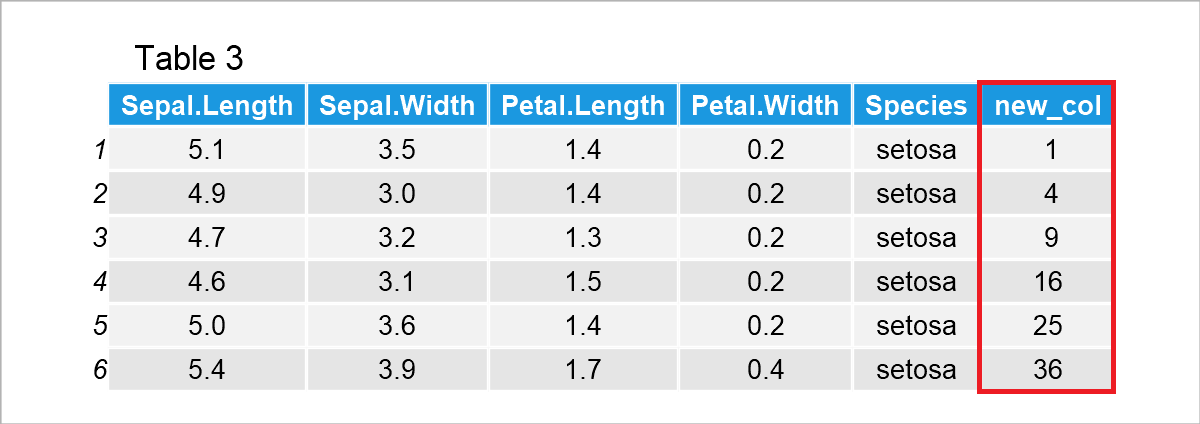
Table 3 illustrates the output of the previous R programming code – A new data frame containing an additional column called new_col.

Example 4: Rename Columns of Data Frame

It is also possible to change the names of the columns of a data frame.

We are using the colnames function for this once again. Furthermore, we are using the paste0 function to create column names with the prefix x and a range from 1 to the number of columns in our data frame (i.e. x1, x2, and so on…).

irisC <- iris                                         # Duplicate data frame
colnames(irisC) <- paste0("x", 1:ncol(irisC))         # Change column names
head(irisC)                                           # Print first six rows of data frame

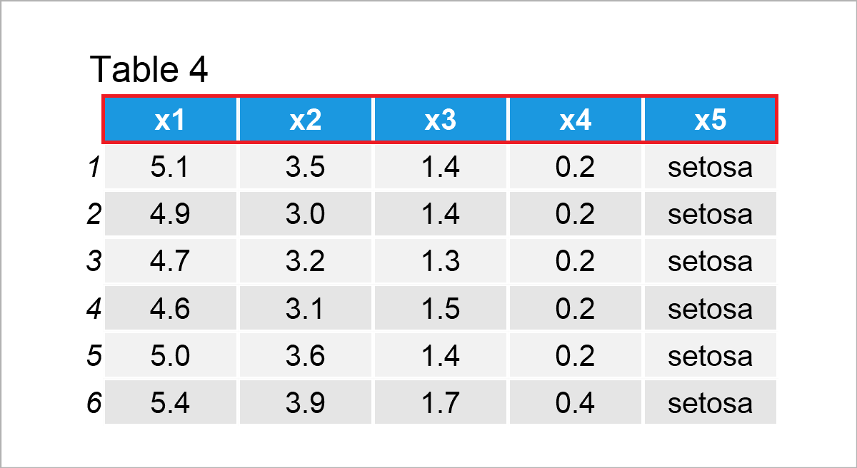
By executing the previously shown syntax, we have created Table 4, i.e. a data frame with renamed variable names.

Example 5: Reorder Rows of Data Frame

Example 5 shows how to order the rows of a data frame.

More precisely, we are sorting our data frame based on the values in the column Sepal.Length by using the order function:

irisD <- iris                                         # Duplicate data frame
irisD <- irisD[order(irisD$Sepal.Length), ]           # Sort rows by values
head(irisD)                                           # Print first six rows of data frame

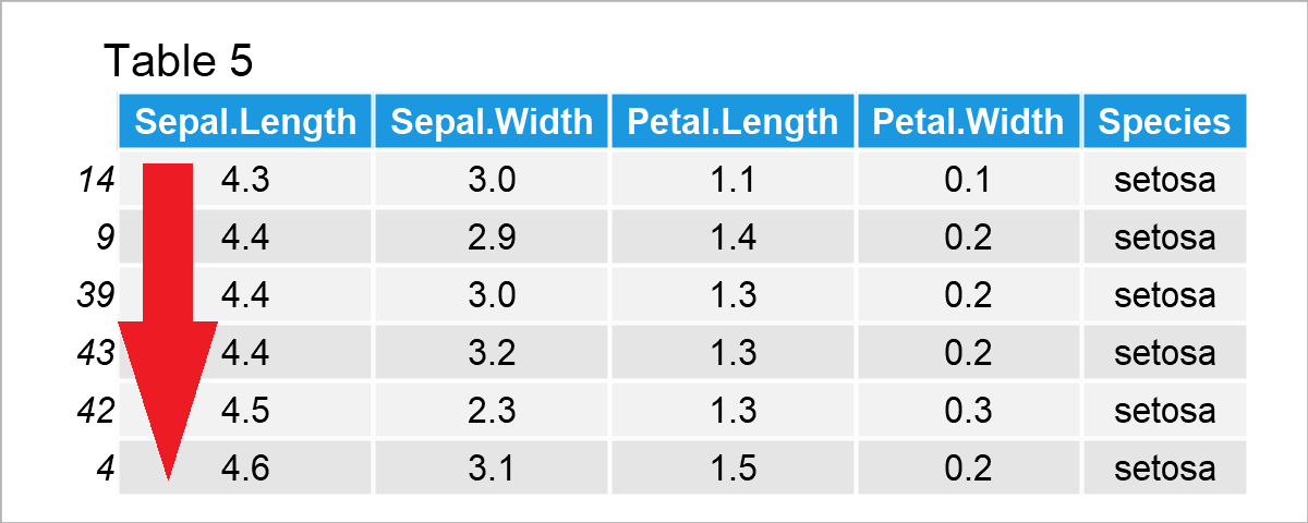
As shown in Table 5, we have created a new version of our data frame where the rows have been sorted based on the column Sepal.Length.

Example 6: Subset Data Frame Rows

Example 6 illustrates how to create a data frame subset by selecting certain rows.

For this task, we can specify the row indices that we want to extract within the c() function:

irisE <- iris                                         # Duplicate data frame
irisE <- irisE[c(1, 3, 5), ]                          # Create data frame subset
irisE                                                 # Print data frame subset

As illustrated in Table 6, we have created a data frame subset using the previous R programming code. This subset contains only three rows of the original input data.

Example 7: Replace Values in Data Frame

In this example, I’ll illustrate how to exchange certain values in a data frame.

Once again, we can use the c() function. In this specific example, I’m exchanging the first, third, and fifth value in the first column by the value 999:

irisF <- iris                                         # Duplicate data frame
irisF[c(1, 3, 5), 1] <- 999                           # Replace values in data frame
head(irisF)                                           # Print first six rows of data frame

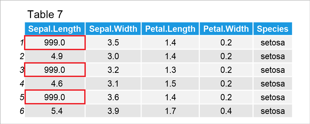
In case you want to replace certain values based on a logical condition, please have a look here.

Example 8: Remove Duplicate Rows in Data Frame

This example shows how to drop duplicate rows from a data frame.

As preparation for this example, we first have to create a data frame with duplicates:

irisG <- rbind(iris[1:3, ], iris[2:5, ])              # Create data frame with duplicates
irisG                                                 # Print data frame with duplicates

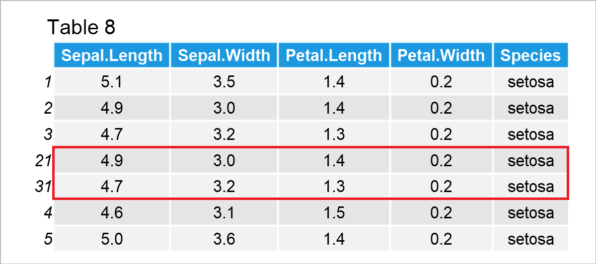
The output of the previously shown R programming code is shown in Table 8. As you can see, the fourth and fifth rows contain the same values as the second and third rows.

If we want to delete these duplicates, we can use the unique function as demonstrated in the following R code:

irisH <- unique(irisG)                                # Drop duplicates from data frame
irisH                                                 # Print data frame with unique rows

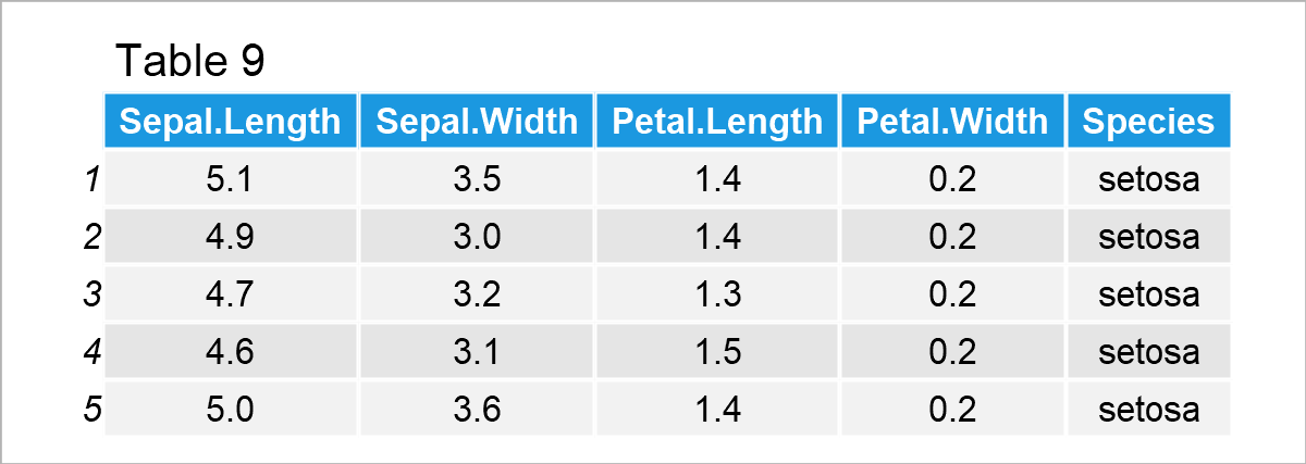
Table 9 reveals the output of the previous R syntax – We have kept only the unique rows in our input data matrix.

Example 9: Aggregate Values in Data Frame by Group

As you might have already noticed, our data frame contains different species groups (or categories). We may use this information to calculate certain descriptive metrics by group.

Example 9 shows how to use the aggregate function to calculate the sum of all the values in the different species groups.

irisI <- aggregate(Sepal.Length ~ Species,            # Calculate sum by group
                   iris,
                   sum)
irisI                                                 # Print sum by group

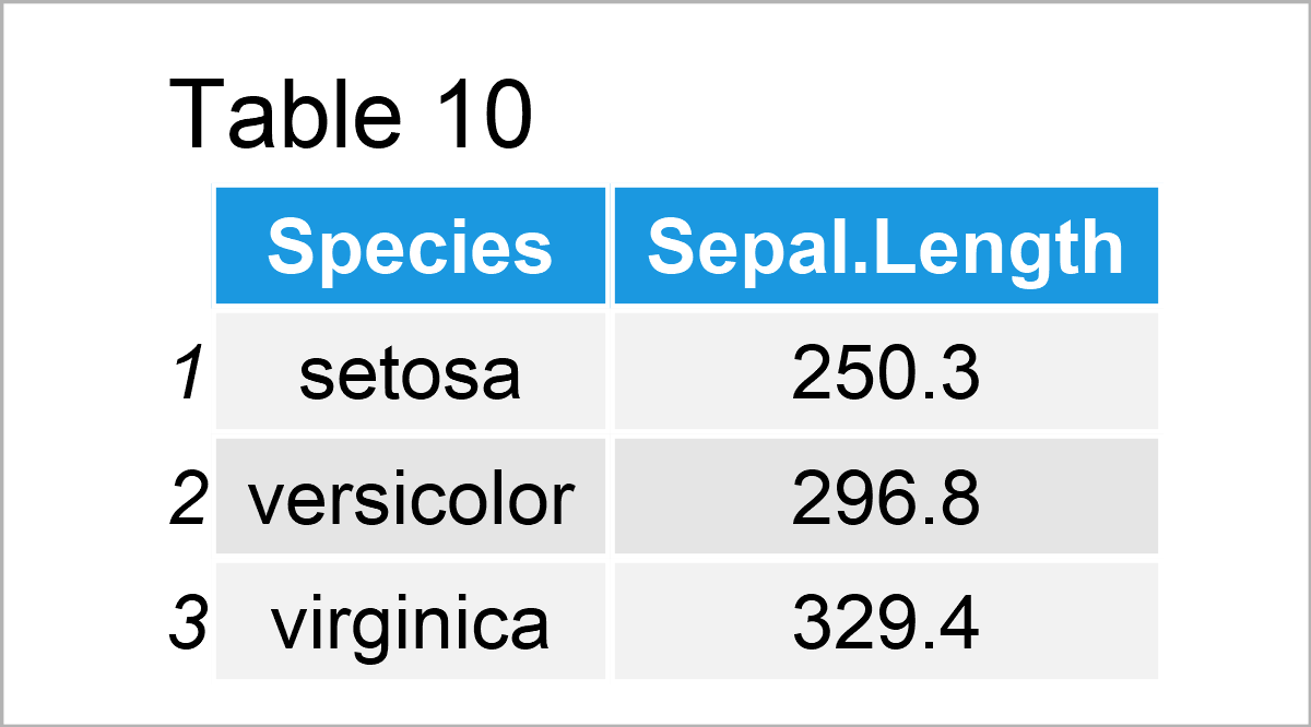
By running the previous syntax, we have managed to construct Table 10, i.e. an aggregated data set showing the sum by group.

Video, Further Resources & Summary

Have a look at the following video on my YouTube channel. I’m showing the examples of this tutorial in the video:

The YouTube video will be added soon.

Besides the video, you may want to have a look at some of the related tutorials on my website. There’s much more to explore in case you want to manipulate, wrangle, and manage data frames in R:

• Data Cleaning in R
• Reshape Data Frame from Wide to Long Format
• Merge Data Frames by Column Names in R
• Remove Rows with Missing Values (i.e. NA) in R
• Working with Complete Cases in R
• Introduction to R

In addition, you may have a look at the dplyr package of the tidyverse and the data.table package. They also provide excellent functions for manipulating and working with data sets – especially for advanced R users.

This tutorial has shown basic and advanced examples on how to edit and handle data frames in the R programming language. Please let me know in the comments section, in case you have further comments and/or questions.