Weibull Distribution in R (4 Examples) | dweibull, pweibull, qweibull & rweibull Functions

In this tutorial you’ll learn how to apply the weibull functions in R.

Table of contents:

Let’s get started:

Example 1: Weibull Density in R (dweibull Function)

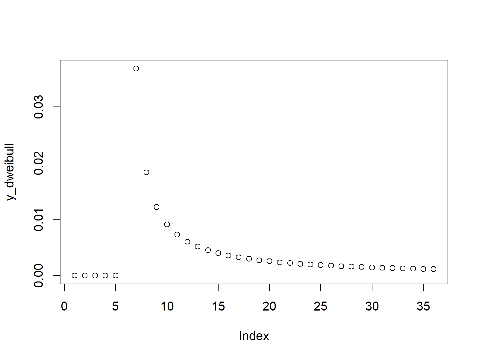
In Example 1, we will create a plot representing the weibull density.

First, we need to create some x-values, for which we want to return the corresponding values of the weibull density:

x_dweibull <- seq(- 5, 30, by = 1)                    # Specify x-values for dweibull function

Now, we can apply the dweibull function of the R programming language to return the corresponding value of the weibull density with a shape of 0.1 and a scale of 1 for each of our input values:

y_dweibull <- dweibull(x_dweibull, shape = 0.1)       # Apply dweibull function

We can create a graphic showing these values with the plot function:

plot(y_dweibull)                                      # Plot dweibull values

weibull density in r

Figure 1: Weibull Density in R Plot.

Figure 1 illustrates the weibull density for a range of input values between -5 and 30 for a shape of 0.1 and a scale of 1.

Example 2: Weibull Distribution Function (pweibull Function)

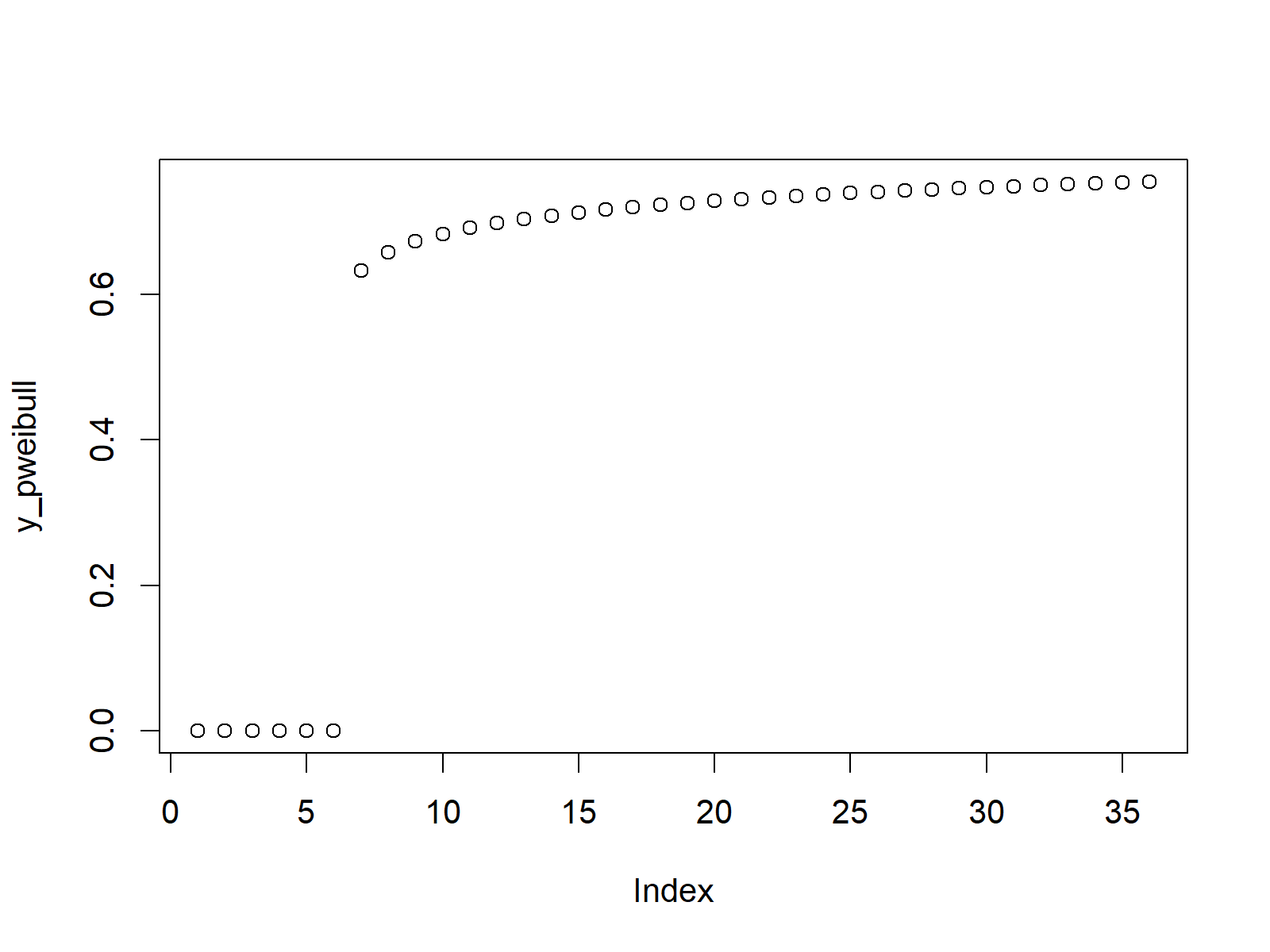
In the second example, we’ll create the cumulative distribution function (CDF) of the weibull distribution.

Again, we need to specify a vector of input values:

x_pweibull <- seq(- 5, 30, by = 1)                    # Specify x-values for pweibull function

Now, we can apply the pweibull R command in order to return the corresponding CDF value for each input value…

y_pweibull <- pweibull(x_pweibull, shape = 0.1)       # Apply pweibull function

…and then we can draw a plot containing these values in R:

plot(y_pweibull)                                      # Plot pweibull values

weibull cdf in r

Figure 2: Cumulative Distribution Function According to Weibull Distribution.

Example 3: Weibull Quantile Function (qweibull Function)

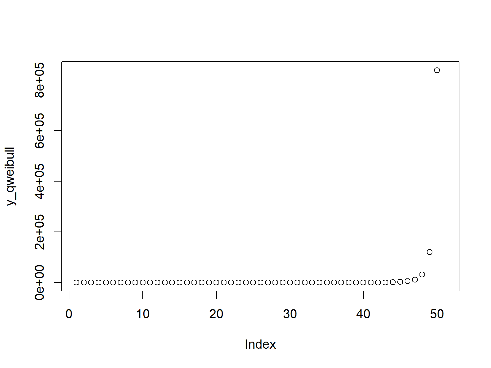
Next, we will create a plot representing the weibull quantile function.

Let’s create a sequence of values between 0 and 1, for which we want to return the corresponding value of the quantile function:

x_qweibull <- seq(0, 1, by = 0.02)                    # Specify x-values for qweibull function

Now, we can use the qweibull R function to return the values of the quantile function:

y_qweibull <- qweibull(x_qweibull, shape = 0.1)       # Apply qweibull function

The following R code produces the corresponding scatterplot:

plot(y_qweibull)                                      # Plot qweibull values

weibull quantile function in r

Figure 3: Weibull Quantile Function.

Example 4: Random Number Generation (rweibull Function)

We can also draw random values according to the weibull density.

First, we need to specify a seed and a sample size of random numbers:

set.seed(13579)                                       # Set seed for reproducibility
N <- 100                                              # Specify sample size

Now, we can use the rweibull command to draw a set of random numbers:

y_rweibull <- rweibull(N, shape = 0.1)                # Draw N weibull distributed values
y_rweibull                                            # Print values to RStudio console
# 2.924615e+03 1.248956e-09 3.362811e+03 1.392134e-10 4.235278e-01 3.332413e+00 2.545625e+04

The RStudio console output is showing the result of the previous R syntax.

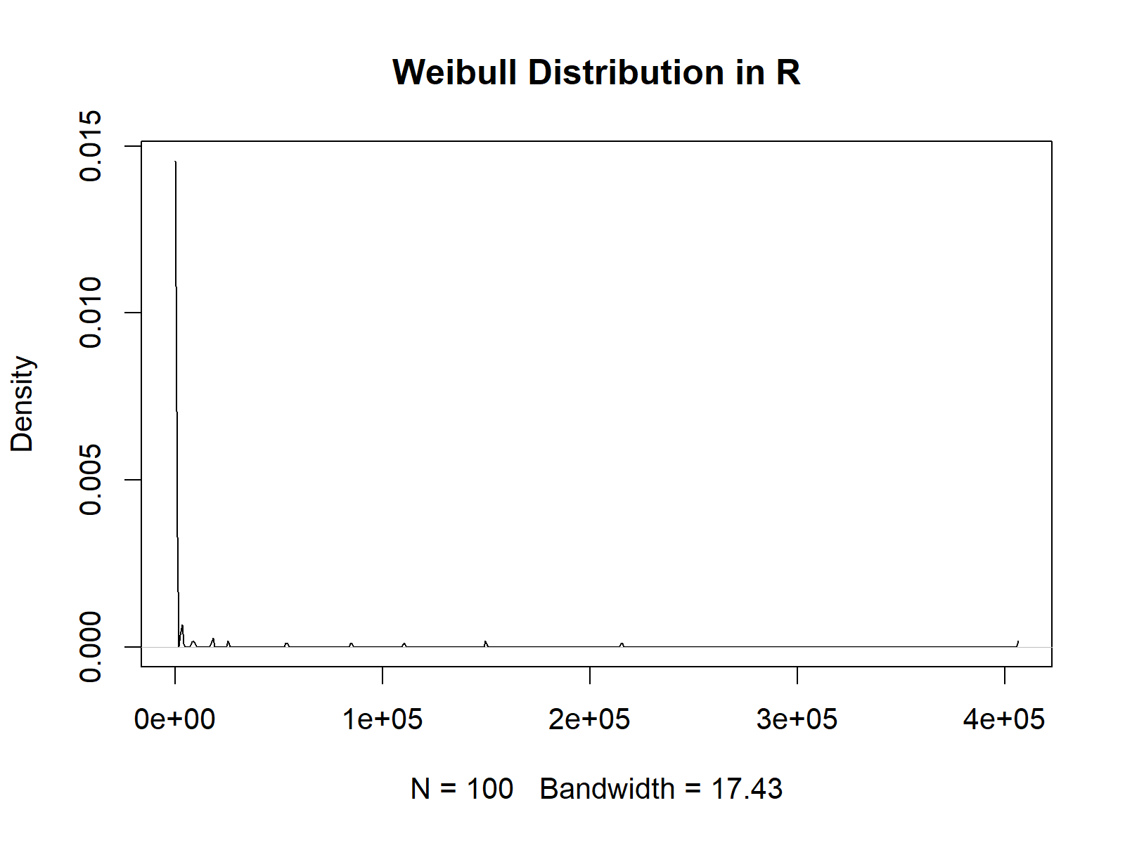
We can also produce a density plot of these numbers:

plot(density(y_rweibull),                             # Plot of randomly drawn weibull density
     main = "Weibull Distribution in R")

random numbers weibull function rweibull

Figure 4: Random Weibull Numbers.

Video, Further Resources & Summary

Do you need more information on the R code of this tutorial? Then you may want to have a look at the following video of my YouTube channel. I’m explaining the R programming codes of this tutorial in the video:

The YouTube video will be added soon.

You could also read the other pages on distributions and the generation of random numbers in R:

Additionally, you may have a look at some of the related articles of this homepage.

In this post you learned some basics of the weibull distribution in R. Don’t hesitate to let me know in the comments section, in case you have additional questions.

6 Comments. Leave new

md3948869
April 26, 2023 2:37 am

x_dweibull <- seq(- 5, 30, by = 1)
y_dweibull <- dweibull(x_dweibull, shape = 0.1)
Can I consider x_dweibull as the observed value and y_dweibull as the predicted value of x_dweibull? Now if I want to find the root mean square of the error (RMSE) using the following code,
library("Metrics")
rmse(x_dweibull, y_dweibull)
I got the result is Inf.
So, my question is: how do I find the RMSE of a Weibull distribution?

Reply
- Cansu (Statistics Globe)
  April 27, 2023 12:44 pm
  Hello,
  
  It seemed to me that it is due to the data you created and how randomly you selected the parameters of distribution. It is possible that that’s why you get an Infinite output. You can try first to fit the Weibull distribution and decide the scaling parameters accordingly, then check the difference between the observed and predicted data. See the example below. I have changed the observed data and how the predicted values are calculated.
  set.seed(42) shape <- 2 scale <- 10 n <- 1000 observed_data <- rweibull(n, shape = shape, scale = scale) #install.packages("fitdistrplus") library("fitdistrplus") fit <- fitdist(observed_data, "weibull") fitted_shape <- fit$estimate["shape"] fitted_scale <- fit$estimate["scale"] predicted_data <- dweibull(n, shape = fitted_shape, scale = fitted_scale) #install.packages("Metrics") library("Metrics") rmse(observed_data, predicted_data)
  Regards,
  Cansu
  Reply
  - md3948869
    April 30, 2023 5:37 am
    
    Thnak u.
    
    Reply
    - Cansu (Statistics Globe)
      May 2, 2023 8:32 am
      
      Very welcome.
      
      Best,
      Cansu
      
      Reply

river735289

May 22, 2023 5:14 pm

Hey,
how can I plot a bimodal weibull-function (two-peaks)? I would like to reproduce the plots from a paper, but I have no data, only the 2 shape and scale parameters and a connection value (g) of the two functions.
scale1 = 9.09
scale2 = 52.30
shape1 = 0.92
shape2 = 2.76
g = 0.73

Thanks a lot!

Cansu (Statistics Globe)

May 23, 2023 8:55 am

Hello!

Could the solution given below be what you are looking for?

# Load required packages
library(ggplot2)
 
# Set the parameters for bimodal Weibull distribution
scale1 <- 9.09
scale2 <- 52.30
shape1 <- 0.92
shape2 <- 2.76
g <- 0.73
 
# Define the bimodal Weibull function
bimodal_weibull <- function(x) {
  density <- g * dweibull(x, scale = scale1, shape = shape1) +
    (1 - g) * dweibull(x, scale = scale2, shape = shape2)
  density
}
 
# Generate x values
x <- seq(0, 100, length.out = 1000)
 
# Calculate the y values using the bimodal Weibull function
y <- bimodal_weibull(x)
 
# Create a data frame for plotting
data <- data.frame(x = x, y = y)
 
# Plot the bimodal Weibull function
ggplot(data, aes(x = x, y = y)) +
  geom_line() +
  xlab("x") +
  ylab("Density")