Half Normal Distribution in R (4 Examples)

This tutorial explains how to use the half normal distribution in R programming.

Table of contents:

Let’s dive right into the examples!

Example Data & Add-On Packages

The following data will be used as a basis for this R tutorial:

x <- seq(0, 10, by = 0.01)               # Specify x-values

We also need to install and load the fdrtool package, in order to use the corresponding functions and commands:

install.packages("fdrtool")              # Install & load fdrtool package
library("fdrtool")

Now, we are set up and can move on to the examples!

Example 1: Half Normal Probability Density Function (dhalfnorm Function)

In this section, I’ll illustrate how to apply the dhalfnorm function to get a half normal probability density.

Have a look at the R code below:

y_dhalfnorm <- dhalfnorm(x)              # Apply dhalfnorm function

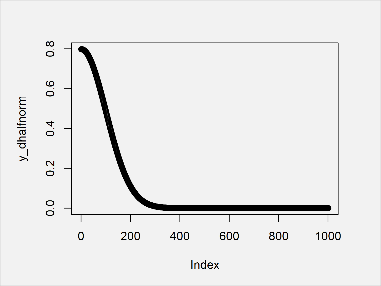
The previous syntax has created a vector of values corresponding to the half normal density.

Let’s draw these data:

plot(y_dhalfnorm)                        # Plot dhalfnorm values

The output of the previous R programming syntax is shown in Figure 1: A half normal density plot.

Example 2: Half Normal Cumulative Distribution Function (phalfnorm Function)

The following R syntax explains how to use the phalfnorm function to get the half normal cumulative distribution.

Once again, we can use our data object x a basis. To this data object, we can apply the phalfnorm function as shown below:

y_phalfnorm <- phalfnorm(x)              # Apply phalfnorm function

Let’s draw this output as well:

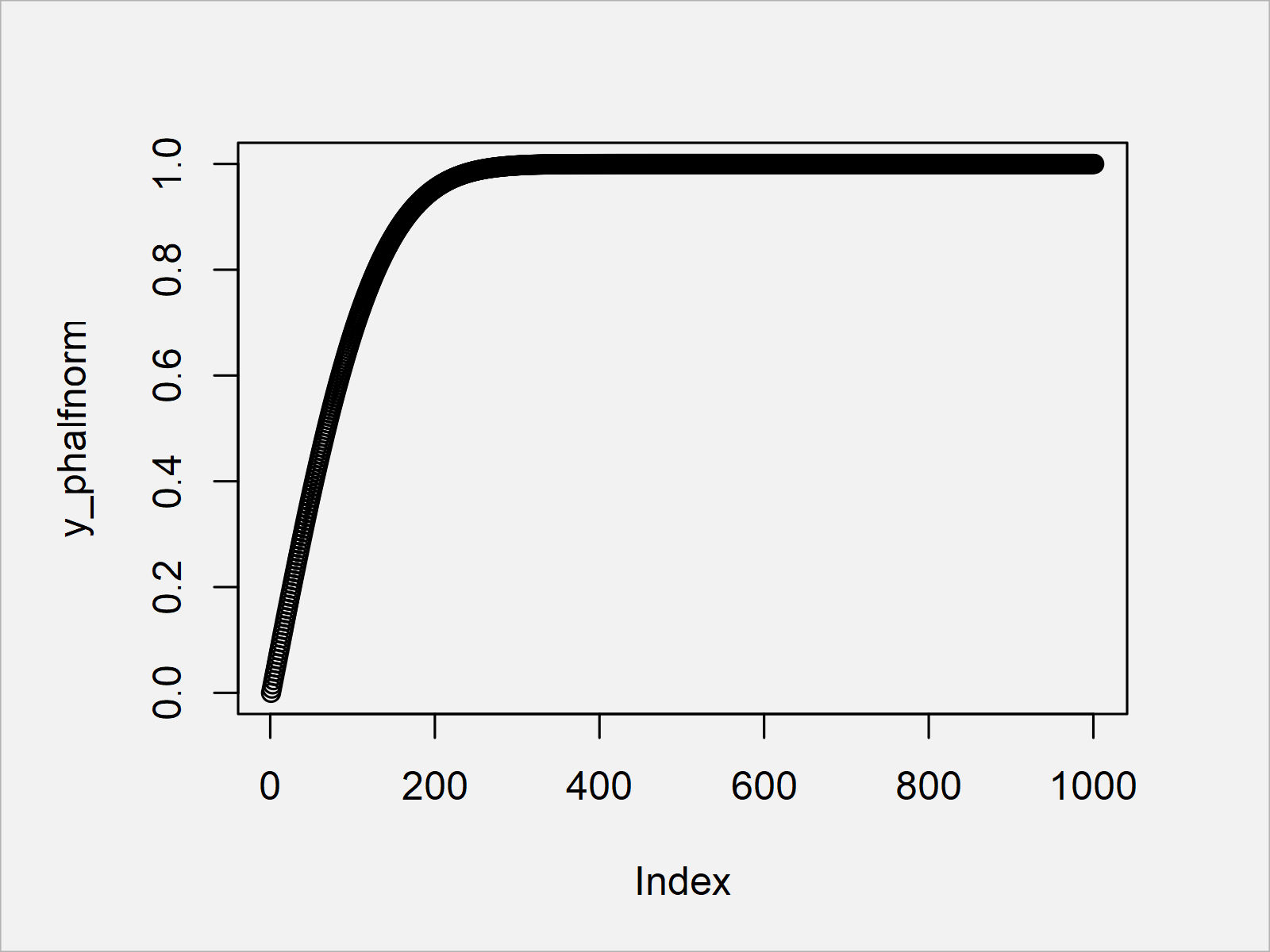
plot(y_phalfnorm)                        # Plot phalfnorm values

By executing the previous R code, we have created Figure 2, i.e. a plot of the half normal cumulative distribution.

Example 3: Half Normal Quantile Function (qhalfnorm Function)

In this example, I’ll show how to use the half normal quantile function in the R programming language.

For this, we first need to create a new x-vector ranging from 0 to 1:

x_qhalfnorm <- seq(0, 1, by = 0.01)      # Specify x-values for qhalfnorm function

Next, we can apply the qhalfnorm function to this vector:

y_qhalfnorm <- qhalfnorm(x_qhalfnorm)    # Apply qhalfnorm function

Let’s plot our new data:

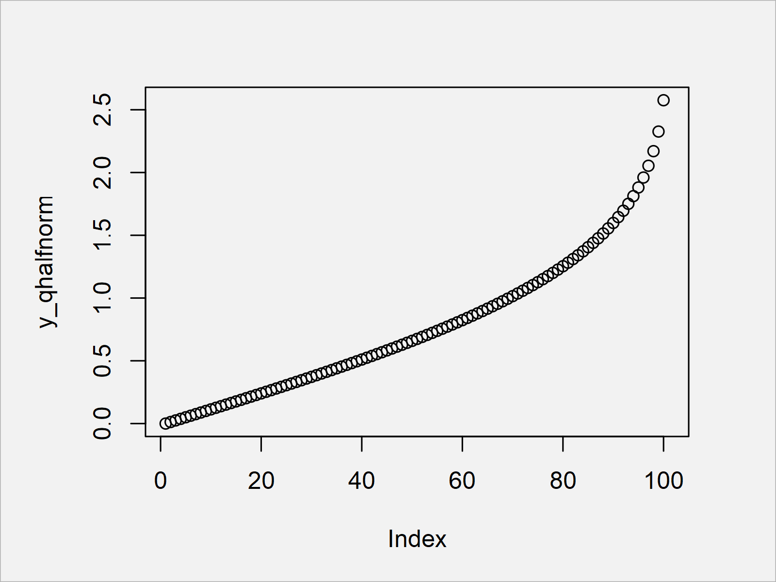
plot(y_qhalfnorm)                        # Plot qhalfnorm values

As shown in Figure 3, we have created a plot of the half normal quantile function by running the previous code.

Example 4: Generating Random Numbers (rhalfnorm Function)

The R programming syntax below demonstrates how to generate random numbers following the half normal distribution.

First, we have to set a random seed, and we have to specify the number of random numbers we want to draw:

set.seed(637452334)                      # Set seed for reproducibility
N <- 10000                               # Specify sample size

Next, we can apply the rhalfnorm function as shown below:

y_rhalfnorm <- rhalfnorm(N)              # Draw N half normally distributed values
head(y_rhalfnorm)                        # Print values to RStudio console
# [1] 1.1599856 0.3692092 0.5849656 0.9449763 2.7898802 1.0108633

Let’s visualize our random data:

hist(y_rhalfnorm,                        # Plot of randomly drawn half normal density
     breaks = 100,
     main = "")

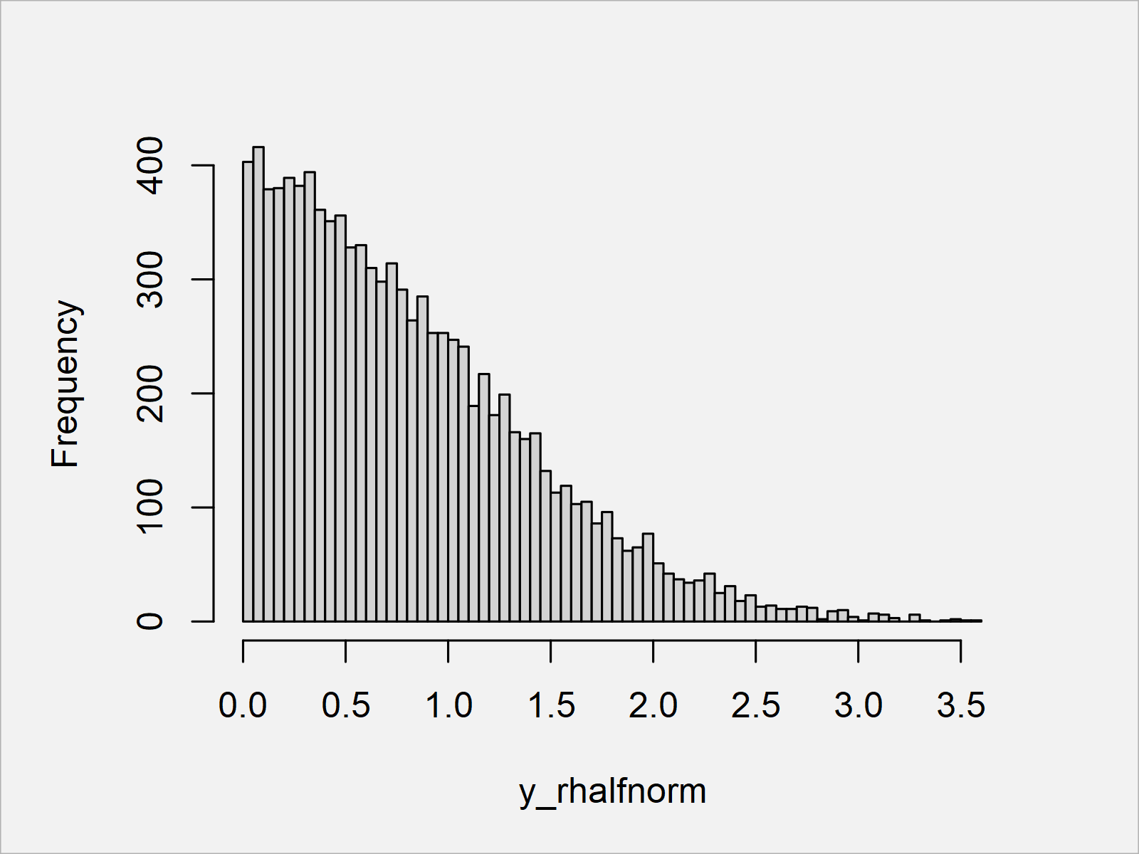
After running the previous code the histogram shown in Figure 4 has been created.

As you can see, our random values are following the half normal distribution.

Video, Further Resources & Summary

Do you want to know more about the usage of the half normal distribution? Then I can recommend having a look at the following video on my YouTube channel. In the video, I’m explaining the examples of this article.

The YouTube video will be added soon.

In addition, you could read the related tutorials on this website. You can find some articles that are related to the usage of the half normal distribution below.

• Log Normal Distribution in R
• Normal Distribution in R
• Simulate Bivariate & Multivariate Normal Distribution
• R Programming Language

You have learned in this article how to deal with the half normal distribution in the R programming language. If you have any further comments or questions, let me know in the comments.