Continuous Uniform Distribution in R (4 Examples) | dunif, punif, qunif & runif Functions

This page explains how to apply the uniform distribution functions in the R programming language.

The content of the post is structured like this:

Let’s take a look at some R codes in action…

Example 1: Uniform Probability Density Function (dunif Function)

In the first example, I’ll show you how a continuous uniform distribution looks like. First, we need to create a vector of quantiles, for which we want to return the corresponding values of the uniform probability density function (PDF):

x_dunif <- seq(0, 100, by = 1)                       # Specify x-values for dunif function

Now, we can use the dunif R command to return the corresponding PDF values of our vector of quantiles. Note that we are specifying the minimum value of the uniform distribution to be 10 and the maximum value to be 50:

y_dunif <- dunif(x_dunif, min = 10, max = 50)        # Apply dunif function

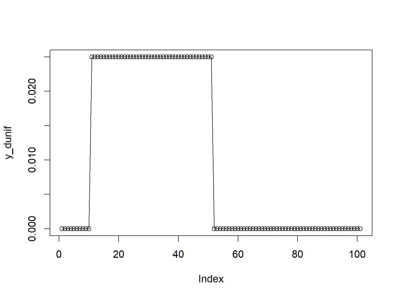
The previous R code created the data object y_dunif containing the PDF values of our uniform distribution. To draw a graphic that shows our uniform density, we can use the plot function as follows:

plot(y_dunif, type = "o")                            # Plot dunif values

uniform probability distribution function (PDF) in the R programming language

Figure 1: R Plot of Uniform Probability Density Function.

Figure 1 shows the output of the previous R syntax. As you can see, our uniform density remains at 0 up to the point 10, (i.e. the minimum value of our uniform distribution). Then it instantly goes up to a probability of 1 and remains at this level until we reach the value 50 (i.e. the maximum of our uniform distribution).

Example 2: Uniform Cumulative Distribution Function (punif Function)

In Example 2 you’ll learn how to create a graphic of the cumulative distribution function of a uniform distribution (CDF). Similar to Example 1, we first have to create a vector of quantiles:

x_punif <- seq(0, 100, by = 1)                       # Specify x-values for punif function

Then, we can apply the punif function to get the corresponding values of the CDF

y_punif <- punif(x_punif, min = 10, max = 50)        # Apply punif function

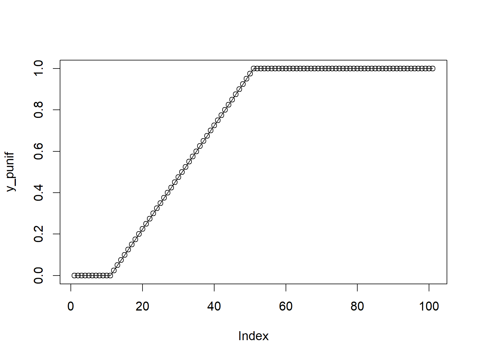
As in Example 1, we can visualize the CDF with the plot function:

plot(y_punif, type = "o")                            # Plot punif values

uniform cumulative distribution function (PDF) in the R programming language

Figure 2: R Plot of Uniform Cumulative Distribution Function.

Example 3: Uniform Quantile Function (qunif Function)

We can draw a quantile function as you can see in the R code below. First, we need to create a sequence of probabilities (i.e. values between 0 and 1):

x_qunif <- seq(0, 1, by = 0.01)                      # Specify x-values for qunif function

To get the corresponding values of the quantile function, we have to apply the qunif R command:

y_qunif <- qunif(x_qunif, min = 10, max = 50)        # Apply qunif function

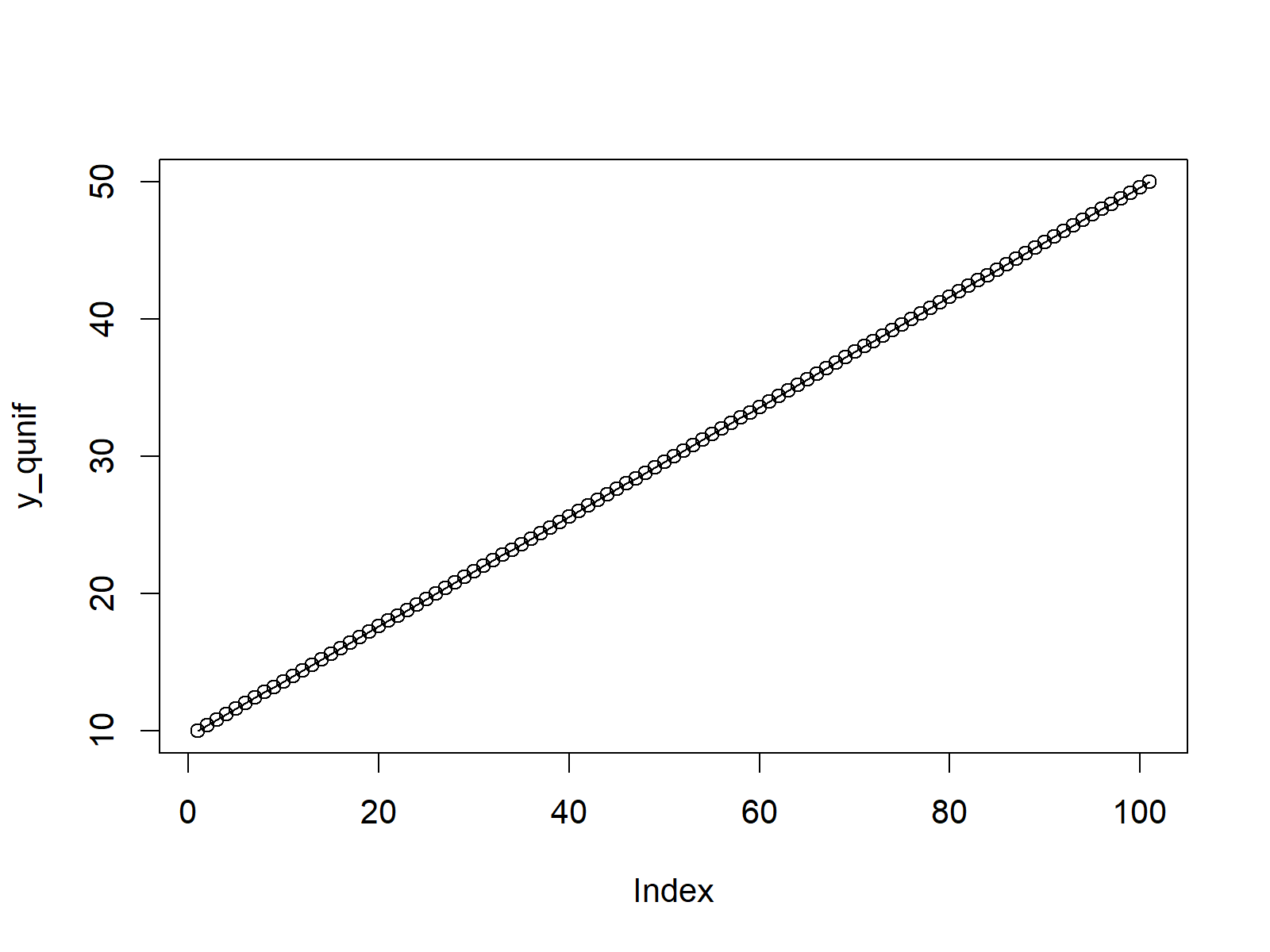
As in the previous examples, we can apply the plot function to draw a graphic of our values:

plot(y_qunif, type = "o")                            # Plot qunif values

uniform quantile function (PDF) in the R programming language

Figure 3: R Plot of Uniform Quantile Function.

Example 4: Generating Random Numbers (runif Function)

We can also simulate a set of uniformly distributed random numbers. To create a reproducible example, we need to specify a seed:

set.seed(91929)                                      # Set seed for reproducibility

Furthermore, we have to specify the sample size of random numbers that we want to generate:

N <- 1000000                                         # Specify sample size

In order to generate a set of random numbers with a uniform distribution, we have to apply the runif function:

y_runif <- runif(N, min = 10, max = 50)              # Draw N uniformly distributed values
y_runif                                              # Print values to RStudio console
# 27.98052 49.43937 24.66723 39.36479 36.84591 40.94262 25.38942 35.59081...

Have a look at the previous output of the RStudio console. It is showing our set of uniformly distributed random numbers.

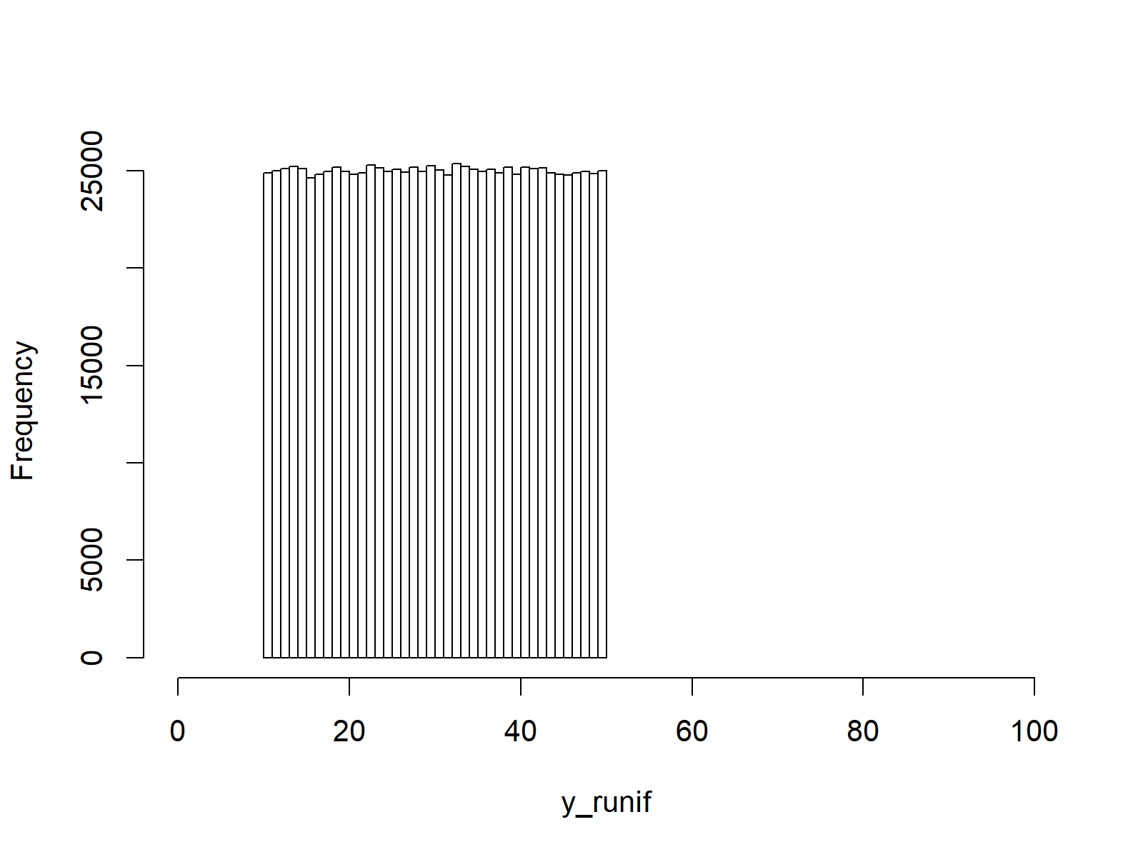
We can illustrate the distribution of our random numbers in a histogram by applying the hist R function:

hist(y_runif,                                        # Plot of randomly drawn uniformly density
     breaks = 50,
     main = "",
     xlim = c(0, 100))

histogram of uniformly distributed random values in R

Figure 4: R Histogram of Uniformly Distributed Random Numbers.

In Figure 4, you can see the distribution of our random numbers: It’s a uniform distribution with a minimum of 10 and a maximum of 50 (i.e. the same distribution as in Example 1).

Video & Further Resources

Would you like to learn more about uniform probability distributions in R? Then you might watch the following video of my YouTube channel. I show the R syntax of this tutorial in the video.

The YouTube video will be added soon.

You may also have a look at the other tutorials on distributions and the generation of random numbers in R:

In addition, you may have a look at the related articles of statisticsglobe.com.

In summary: At this point of the article you should have learned how to draw and simulate a uniform distribution in the R programming language. Let me know in the comments section, if you have further questions.