Beta Distribution in R (4 Examples) | dbeta, pbeta, qbeta & rbeta Functions

This article shows how to use the beta functions in R programming.

The content of the page looks as follows:

• Example 1: Beta Density in R (dbeta Function)
• Example 2: Beta Distribution Function (pbeta Function)
• Example 3: Beta Quantile Function (qbeta Function)
• Example 4: Random Number Generation (rbeta Function)
• Video & Further Resources

If you want to know more about these topics, keep reading:

Example 1: Beta Density in R (dbeta Function)

The dbeta R command can be used to return the corresponding beta density values for a vector of quantiles.

Let’s create such a vector of quantiles in R:

x_beta <- seq(0, 1, by = 0.02)                     # Specify x-values for beta function

Now, we can apply the dbeta function to return the values of the beta density that correspond to our input vector and the two shape parameters shape1 and shape2 (i.e. 2 and 5):

y_beta <- dbeta(x_beta, shape1 = 2, shape2 = 5)    # Apply beta function

We can also create a graphic in R, which shows our previously created values:

plot(y_beta)                                       # Plot beta values

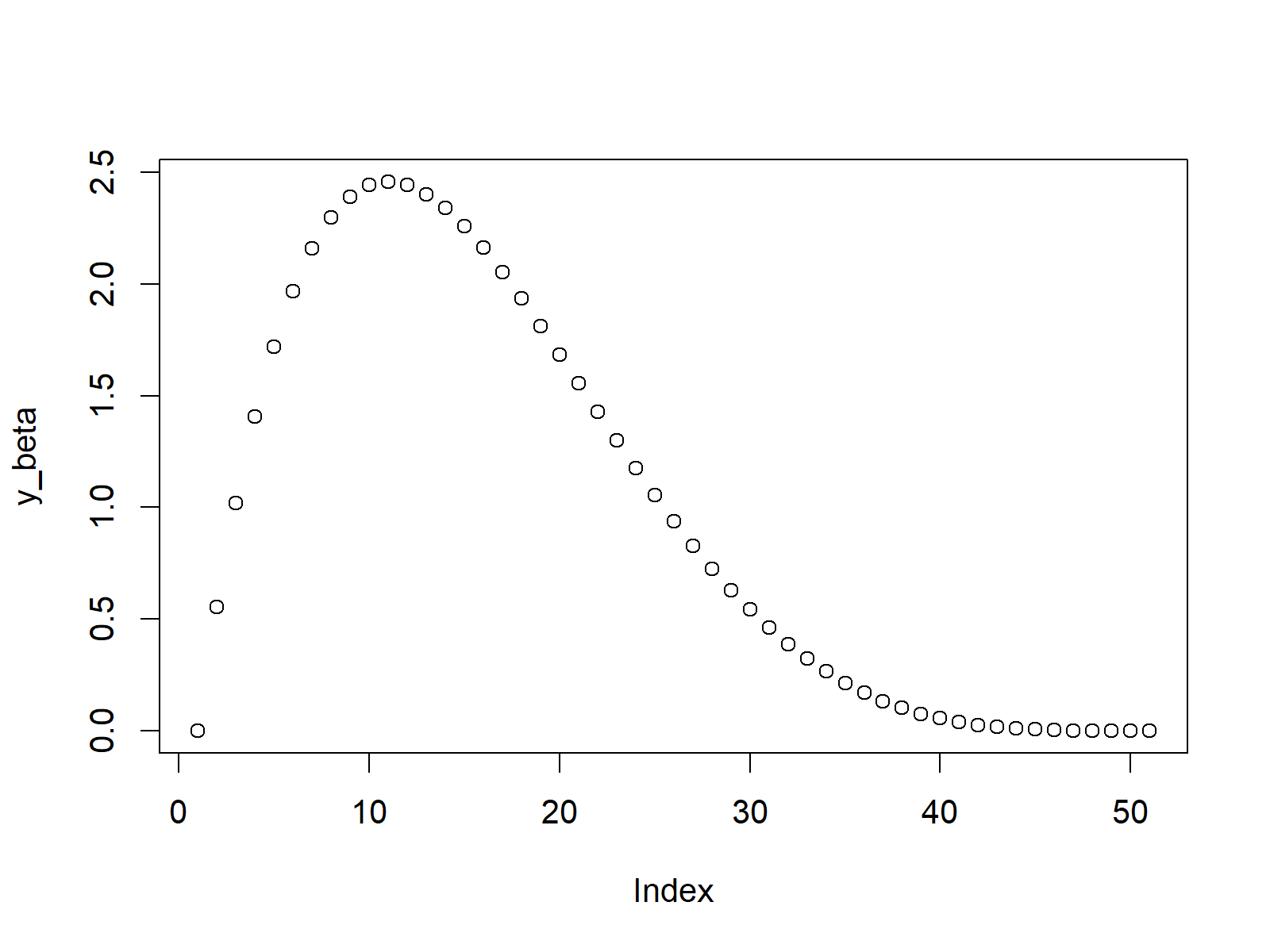
Figure 1: Beta Density in R.

Example 2: Beta Distribution Function (pbeta Function)

In the second example, we will draw a cumulative distribution function of the beta distribution. For this task, we also need to create a vector of quantiles (as in Example 1):

x_pbeta <- seq(0, 1, by = 0.02)                    # Specify x-values for pbeta function

This vector of quantiles can now be inserted into the pbeta function:

y_pbeta <- pbeta(x_pbeta, shape1 = 1, shape2 = 5)  # Apply pbeta function

The output is shown in the following graph:

plot(y_pbeta)                                      # Plot pbeta values

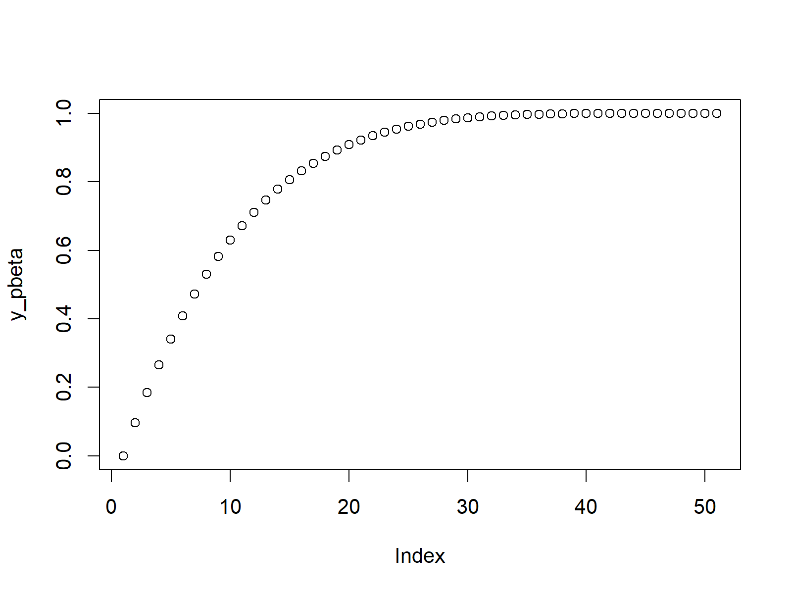
Figure 2: Cumulative Distribution Function of Beta Distribution.

Example 3: Beta Quantile Function (qbeta Function)

The R programming language also provides the possibility to return the values of the beta quantile function. This time we need to create sequence of probabilities as input:

x_qbeta <- seq(0, 1, by = 0.02)                    # Specify x-values for qbeta function

These probabilities can now be inserted into the qbeta function:

y_qbeta <- qbeta(x_qbeta, shape1 = 1, shape2 = 5)  # Apply qbeta function

The following R code produces the corresponding R plot:

plot(y_qbeta)                                      # Plot qbeta values

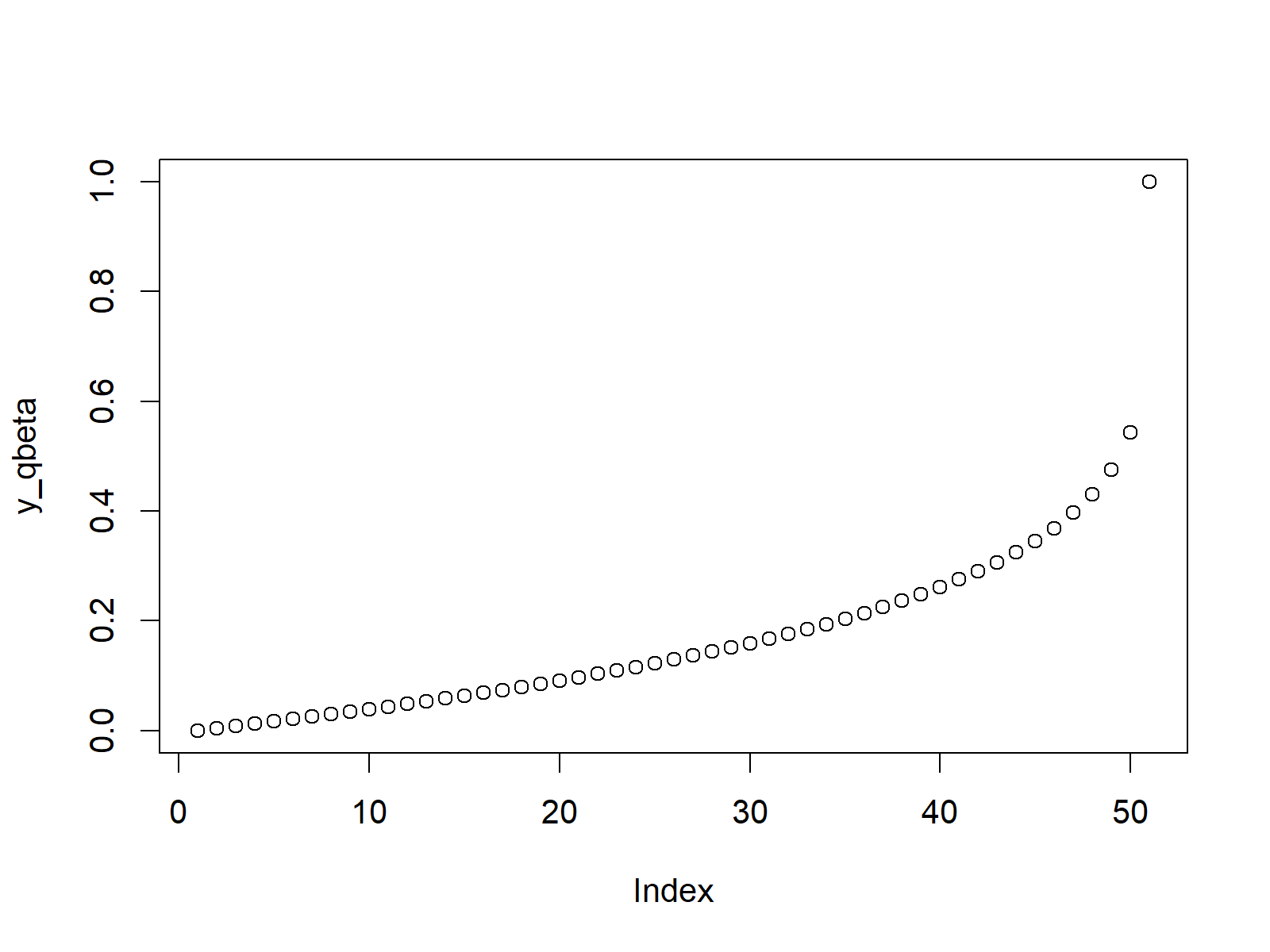
Figure 3: Beta Quantile Function.

Example 4: Random Number Generation (rbeta Function)

In case we want to generate random numbers from the beta density, we need to set a seed and specify our desired sample size first:

set.seed(13579)                                    # Set seed for reproducibility
N <- 10000                                         # Specify sample size

Now, we can use the rbeta function to simulate a set of random numbers drawn from the beta distribution:

y_rbeta <- rbeta(N, shape1 = 1, shape2 = 5)        # Draw N beta distributed values
y_rbeta                                            # Print values to RStudio console
# 0.2311784008 0.0305951096 0.0527656109 0.1289216944 0.2317310221 0.0557187181 0.0855674210 0.4125831741 0.2879114830...

The RStudio console is showing the output of the rbeta function. Let’s plot these values in a density plot:

plot(density(y_rbeta),                             # Plot of randomly drawn beta density
     main = "beta Distribution in R")

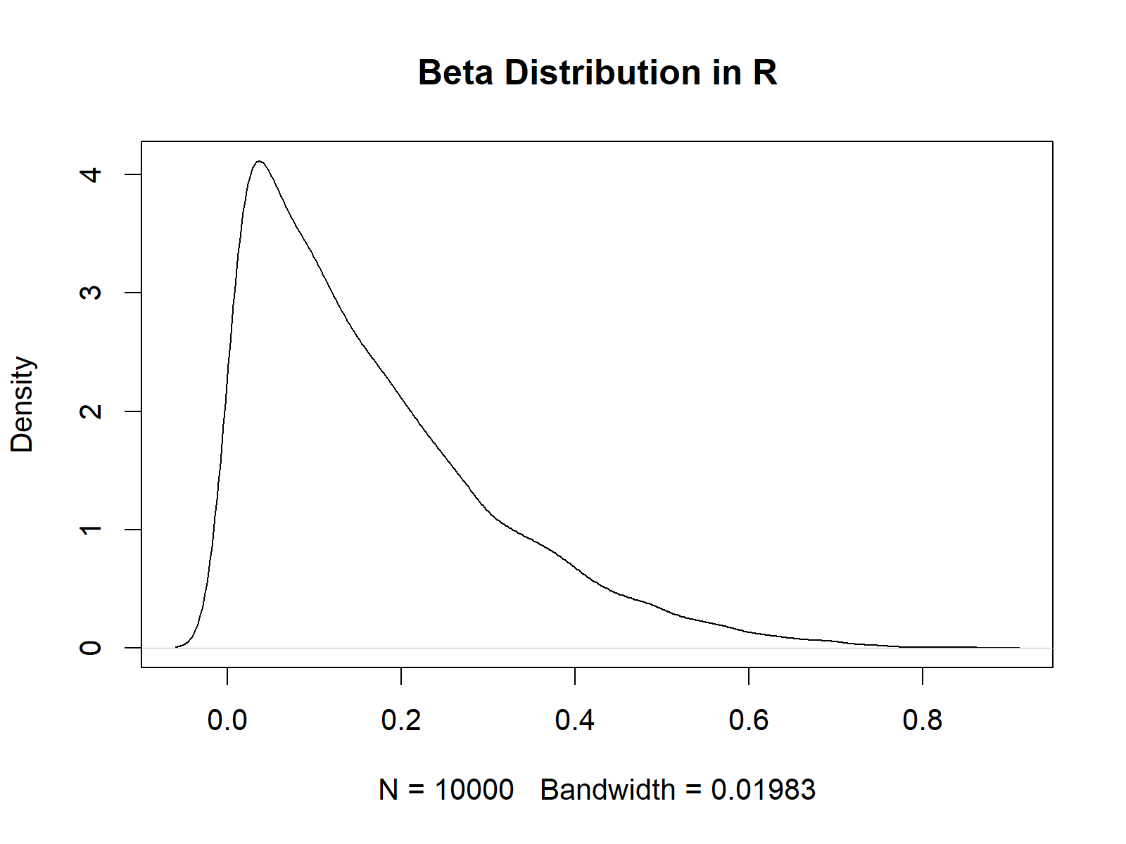
Figure 4: Random Numbers Drawn from Beta Density.

Video & Further Resources

In case you need more information on the R programming codes of this article, I can recommend to have a look at the following video of my YouTube channel. I show the R syntax of this post in the video:

The YouTube video will be added soon.

You could also read the other articles on probability distributions and the simulation of random numbers in R:

• Bernoulli Distribution in R
• Beta Distribution in R
• Binomial Distribution in R
• Bivariate & Multivariate Distributions in R
• Cauchy Distribution in R
• Chi-Squred Distribution in R
• Exponential Distribution in R
• F Distribution in R
• Gamma Distribution in R
• Geometric Distribution in R
• Hypergeometric Distribution in R
• Log Normal Distribution in R
• Logistic Distribution in R
• Negative Binomial Distribution in R
• Normal Distribution in R
• Poisson Distribution in R
• Student t Distribution in R
• Studentized Range Distribution in R
• Uniform Distribution in R
• Weibull Distribution in R
• Wilcoxon Signedank Statistic Distribution in R
• Wilcoxonank Sum Statistic Distribution in R

Also, you could have a look at the related tutorials on this website.

• R Graphics Gallery
• R Functions List (+ Examples)
• The R Programming Language

Summary: In this tutorial, I illustrated how to calculate and simulate a beta distribution in R programming. Tell me about it in the comments below, in case you have any further comments or questions.