Log Normal Distribution in R (4 Examples) | dlnorm, plnorm, qlnorm & rlnorm Functions
This tutorial shows how to apply the log normal functions in R.
The page consists of this content:
- Example 1: Log Normal Probability Density Function (dlnorm Function)
- Example 2: Log Normal Cumulative Distribution Function (plnorm Function)
- Example 3: Log Normal Quantile Function (qlnorm Function)
- Example 4: Generating Random Numbers (rlnorm Function)
- Video & Further Resources
Let’s dig in!
Example 1: Log Normal Probability Density Function (dlnorm Function)
In the first example, I’ll show you how the log normal density looks like. First, we need to create a sequence of quantile values that we can use as input for the dlnorm R function.
x_dlnorm <- seq(0, 10, by = 0.01) # Specify x-values for dlnorm function
Now, we can apply the dlnorm function as follows:
y_dlnorm <- dlnorm(x_dlnorm) # Apply dlnorm function
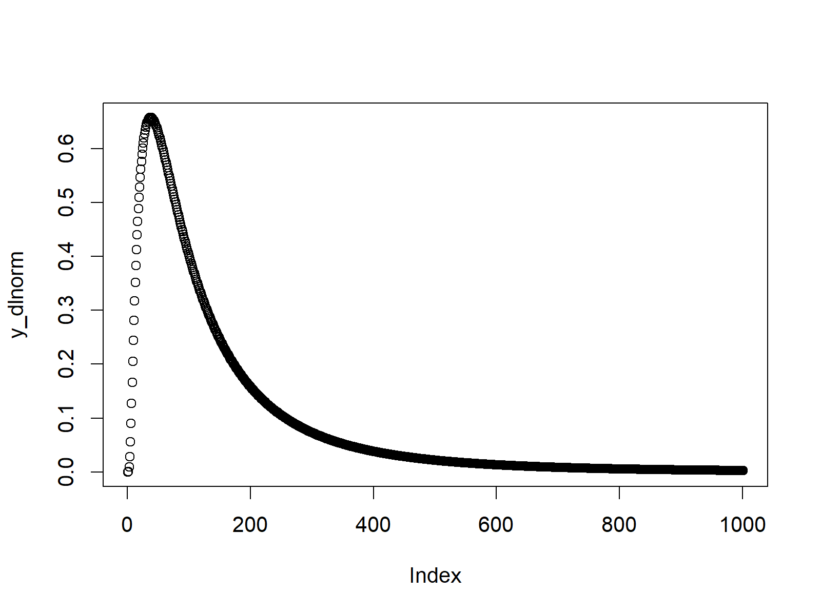
The previous R code stored the output of the dlnorm function in the data object y_dlnorm. We can now use the plot function to draw a graphic, representing the probability density function (PDF) of the log normal distribution:
plot(y_dlnorm) # Plot dlnorm values

Figure 1: PDF of Log Normal Distribution.
Example 2: Log Normal Cumulative Distribution Function (plnorm Function)
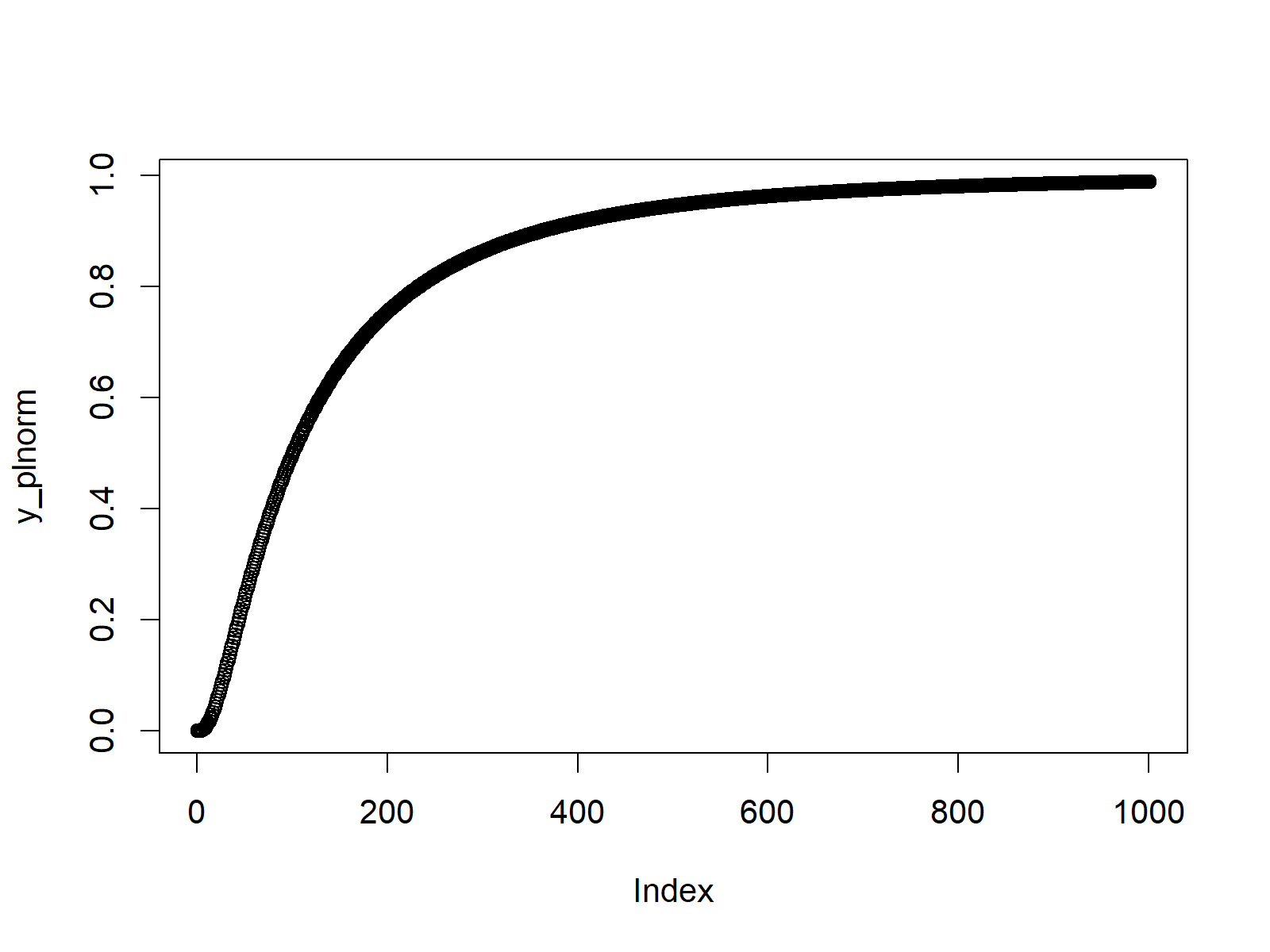
Example 2 shows how to draw the cumulative distribution function (CDF) of the log normal distribution. Again, we need to create a vector of quantiles:
x_plnorm <- seq(0, 10, by = 0.01) # Specify x-values for plnorm function
And then, we need to insert this vector into the plnorm command:
y_plnorm <- plnorm(x_plnorm) # Apply plnorm function
We can draw the cumulative distribution function as follows:
plot(y_plnorm) # Plot plnorm values

Figure 2: CDF of Log Normal Distribution.
Example 3: Log Normal Quantile Function (qlnorm Function)
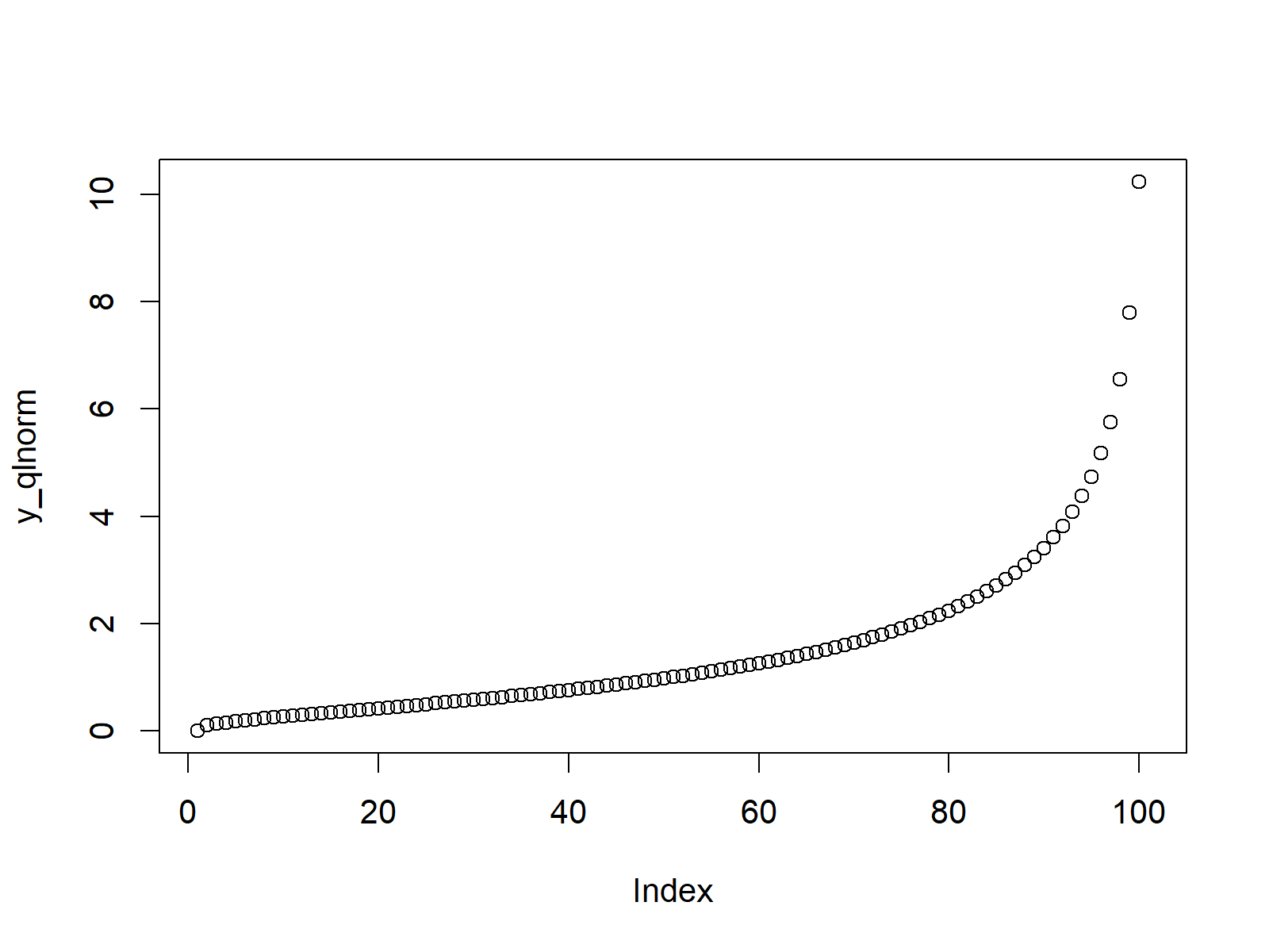
In Example 3, we’ll create the quantile function of the log normal distribution. As a first step, we have to create a sequence of probabilities (i.e. values between 0 and 1):
x_qlnorm <- seq(0, 1, by = 0.01) # Specify x-values for qlnorm function
Then, we can apply the qlnorm function to this sequence:
y_qlnorm <- qlnorm(x_qlnorm) # Apply qlnorm function
Finally, we can draw our quantile function plot of the log normal distribution:
plot(y_qlnorm) # Plot qlnorm values

Figure 3: Quantile Function of Log Normal Distribution.
Example 4: Generating Random Numbers (rlnorm Function)
In the last example of this R tutorial, I’ll explain how to draw random numbers according to the distribution of the log normal density. First, we need to set a seed and specify the amount of random numbers that we want to simulate:
set.seed(91929)                                         # Set seed for reproducibility
N <- 10000                                              # Specify sample size
Then, we can apply the rlnorm function in order to generate N random numbers:
y_rlnorm <- rlnorm(N)                                   # Draw N log normally distributed values
y_rlnorm                                                # Print values to RStudio console
# 0.88082919  0.71130233  1.55750385  0.74597213  1.12296291  1.73100566  0.72801951  1.25833372  2.09056650...
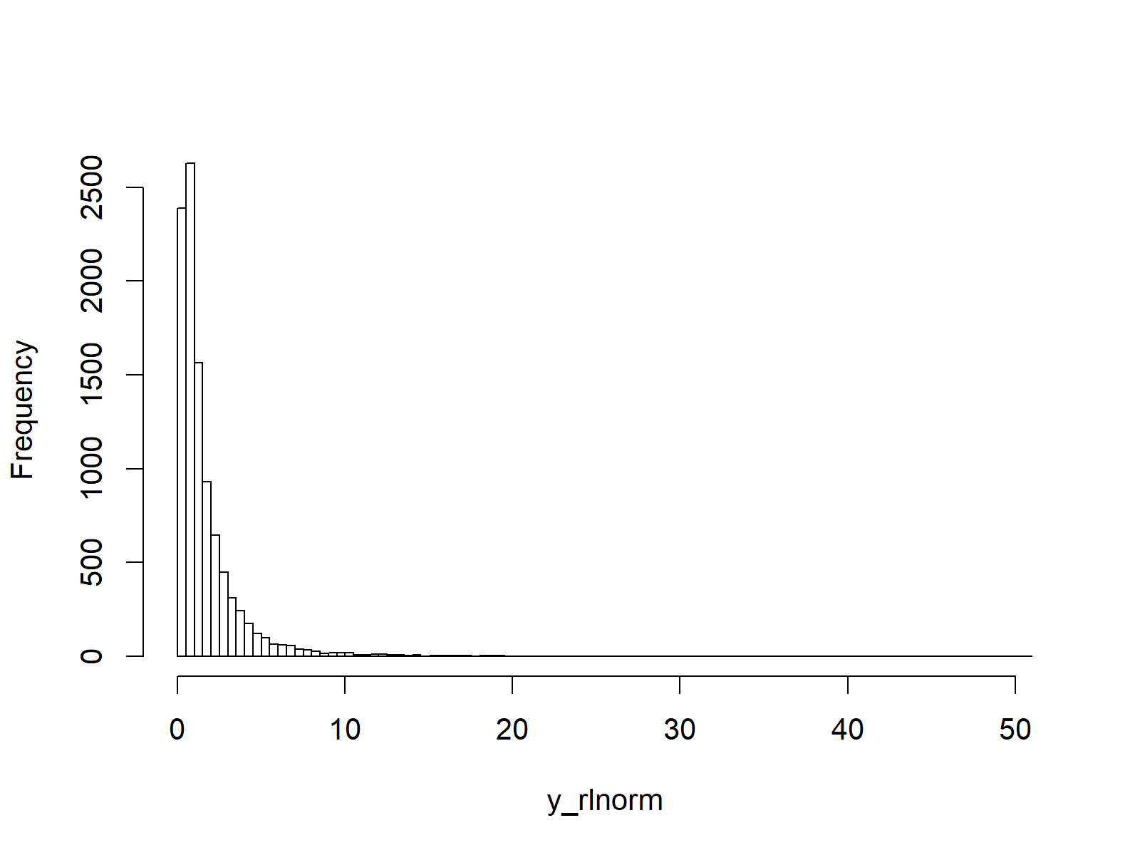
As you can see based on the previous RStudio console output, our random numbers are stored in the data object y_rlnorm. We can draw a histogram showing the distribution of these random numbers as shown below:
hist(y_rlnorm,                                          # Plot of randomly drawn log normal density
     breaks = 100,
     main = "")

Figure 4: Random Numbers Distributed as Log Normal Distribution.
As you can see: The random numbers are distributed as the log normal distribution. Looks fine!
Video & Further Resources
In case you need more info on the R programming syntax of this page, I can recommend to watch the following video of my YouTube channel. I show the examples of this tutorial in the video:
The YouTube video will be added soon.
You might also read the other articles on probability distributions and the simulation of random numbers in R:
- Bernoulli Distribution in R
- Beta Distribution in R
- Binomial Distribution in R
- Bivariate & Multivariate Distributions in R
- Cauchy Distribution in R
- Chi-Squred Distribution in R
- Exponential Distribution in R
- F Distribution in R
- Gamma Distribution in R
- Geometric Distribution in R
- Hypergeometric Distribution in R
- Log Normal Distribution in R
- Logistic Distribution in R
- Negative Binomial Distribution in R
- Normal Distribution in R
- Poisson Distribution in R
- Student t Distribution in R
- Studentized Range Distribution in R
- Uniform Distribution in R
- Weibull Distribution in R
- Wilcoxon Signedank Statistic Distribution in R
- Wilcoxonank Sum Statistic Distribution in R
In addition to the video, I can recommend to read the other articles on my website:
This tutorial illustrated how to use the log normal functions in R programming. Please tell me about it in the comments section, if you have further questions.
Subscribe to the Statistics Globe Newsletter
Get regular updates on the latest tutorials, offers & news at Statistics Globe.
I hate spam & you may opt out anytime: Privacy Policy.
Thank you!
Welcome to the Statistics Globe newsletter. From now on, I’ll send you regular emails about statistics, data science, AI, and programming with R and Python.
I’m Joachim Schork. On this website, I provide statistics tutorials as well as code in Python and R programming.
Statistics Globe Newsletter
Get regular updates on the latest tutorials, offers & news at Statistics Globe. I hate spam & you may opt out anytime: Privacy Policy.
Thank you!
Please check your email inbox and click the confirmation link to complete your subscription. If you don’t see the email within a few minutes, please also check your spam/junk folder.


