Binomial Distribution in R (4 Examples) | dbinom, pbinom, qbinom & rbinom Functions
In this tutorial you’ll learn how to apply the binom functions in R programming.
The tutorial is structured as follows:
- Example 1: Binomial Density in R (dbinom Function)
- Example 2: Binomial Cumulative Distribution Function (pbinom Function)
- Example 3: Binomial Quantile Function (qbinom Function)
- Example 4: Simulation of Random Numbers (rbinom Function)
- Video, Further Resources & Summary
Let’s take a look at some R codes in action!
Example 1: Binomial Density in R (dbinom Function)
In the first example, we’ll create an R plot of the binomial density.
First, we have to create a vector of quantiles as input for the dbinom R function:
x_dbinom <- seq(0, 100, by = 1) # Specify x-values for binom function
Then, we can apply the dbinom function to this vector as shown below. Note that I have specified the size to be equal to 100 (i.e. the number of trials) and the probability for each binomial draw to be equal to 0.5 (i.e. 50%). Of cause you can modify these arguments as you want.
y_dbinom <- dbinom(x_dbinom, size = 100, prob = 0.5) # Apply dbinom function
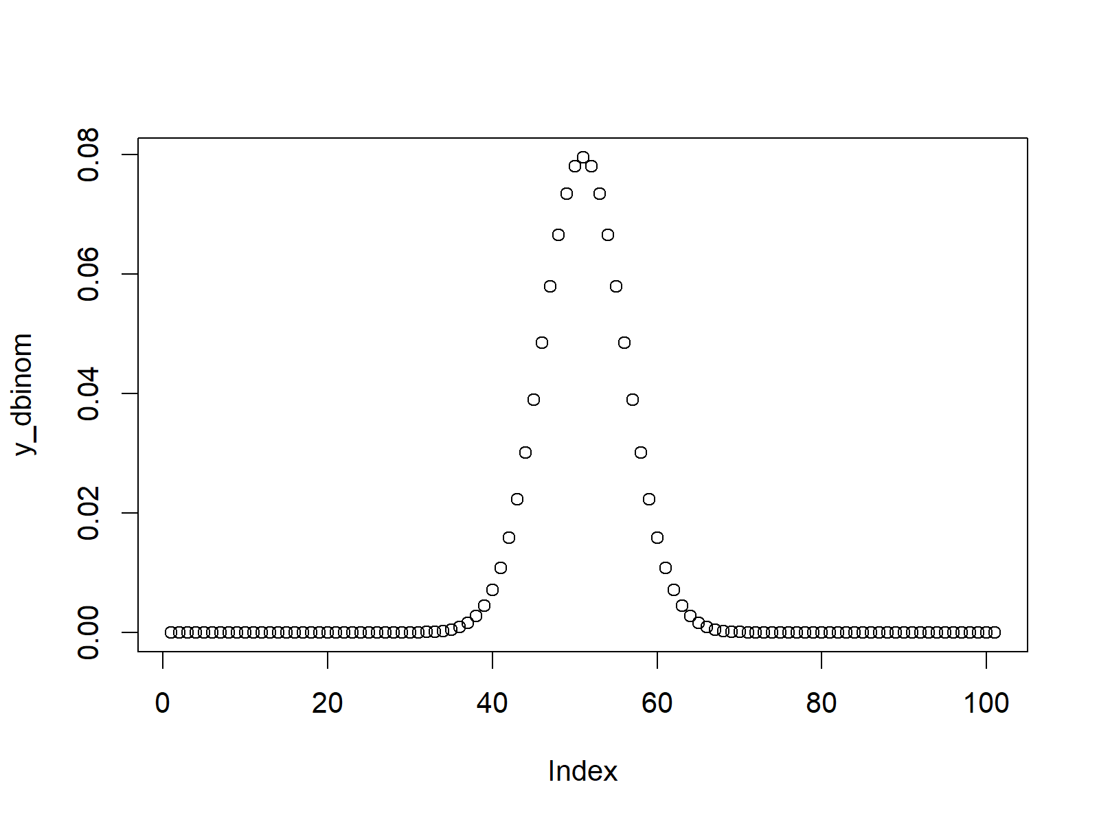
If we want to illustrate the output of the dbinom function in a graphic, we can use the plot function:
plot(y_dbinom) # Plot dbinom values

Figure 1: Binomially Distributed Density.
Figure 1 shows the output of the previous R code – A binomially distributed density.
Example 2: Binomial Cumulative Distribution Function (pbinom Function)
In Example 2, I’ll explain how to apply the pbinom function to create a plot of the binomial cumulative distribution function (CDF) in R. First, we need to create an input vector (as in Example 1).
x_pbinom <- seq(0, 100, by = 1) # Specify x-values for pbinom function
Now, we can apply the pbinom command…
y_pbinom <- pbinom(x_pbinom, size = 100, prob = 0.5) # Apply pbinom function
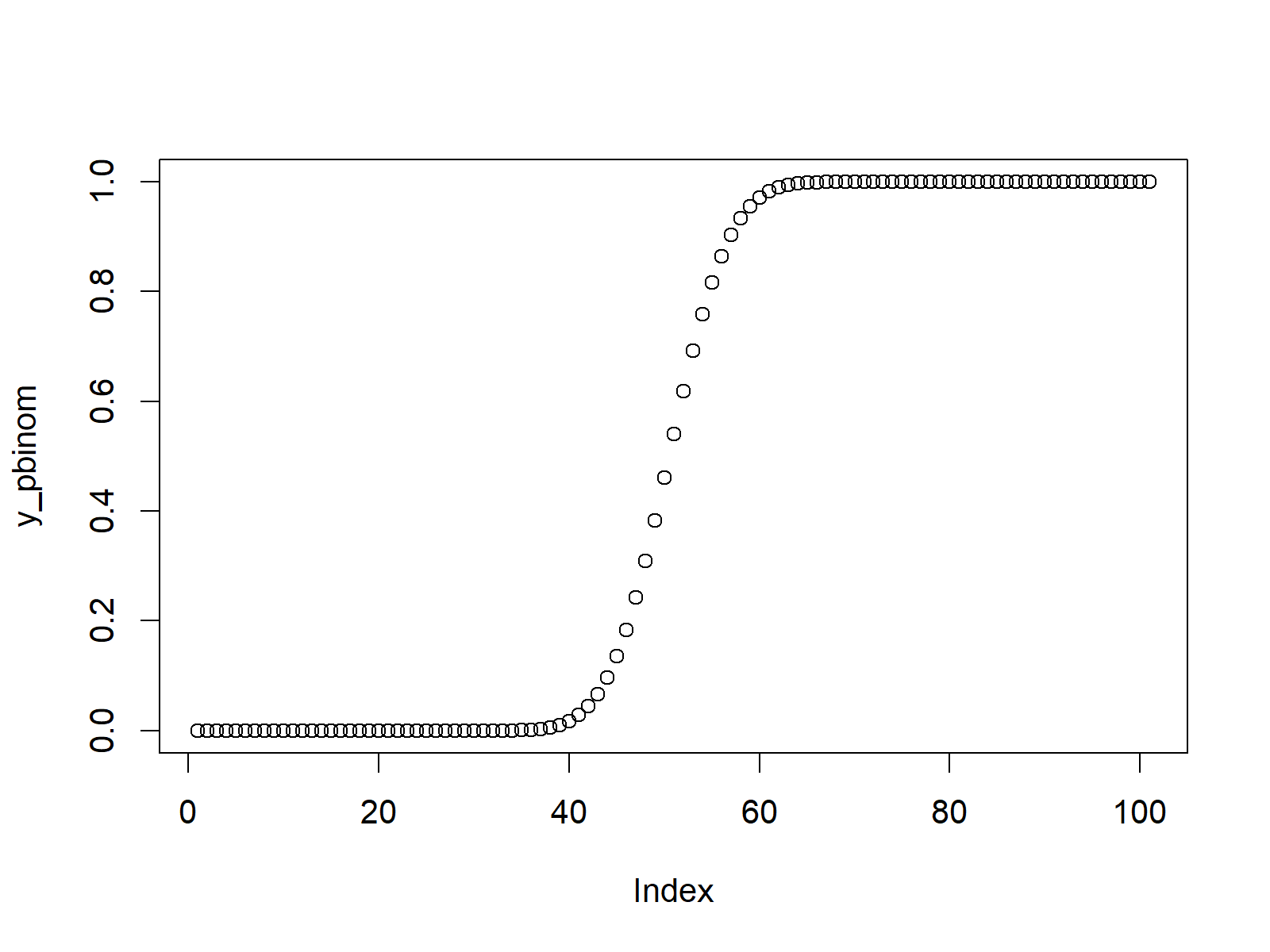
…and draw a plot of the binomial CDF:
plot(y_pbinom) # Plot pbinom values

Figure 2: Binomial CDF in R.
Example 3: Binomial Quantile Function (qbinom Function)
In this example, you’ll learn how to plot the binomial quantile function in R. As a first step, we have to create a sequence of probabilities:
x_qbinom <- seq(0, 1, by = 0.01) # Specify x-values for qbinom function
Then, we can apply the qbinom function to get the corresponding value of the binomial quantile function for each value in our sequence of probabilities:
y_qbinom <- qbinom(x_qbinom, size = 100, prob = 0.5) # Apply qbinom function
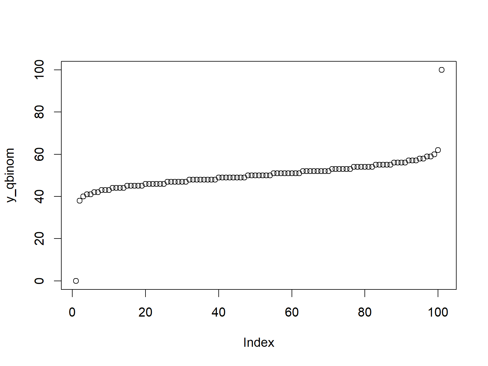
Finally, we can illustrate the output in an R plot:
plot(y_qbinom) # Plot qbinom values

Figure 3: Quantile Function of Binomial Distribution.
Example 4: Simulation of Random Numbers (rbinom Function)
If we want to generate some random numbers with a binomial distribution in R, we can use the rbinom function. Let’s specify a seed for reproducibility…
set.seed(13579) # Set seed for reproducibility
…and a sample size of random numbers that we want to draw:
N <- 10000 # Specify sample size
Now, we can create a set of random numbers with a binomial distribution based on the rbinom function:
y_rbinom <- rbinom(N, size = 100, prob = 0.5)         # Draw N binomially distributed values
y_rbinom                                              # Print values to RStudio console
# 45 44 55 43 35 47 56 52 49 51 47 50 51 54 53 48 57 55 51...
The RStudio console shows the random numbers that we have just created. They have a (theoretical) range between 0 and 100 (i.e. 0 positive outcomes or 100 positive outcomes).
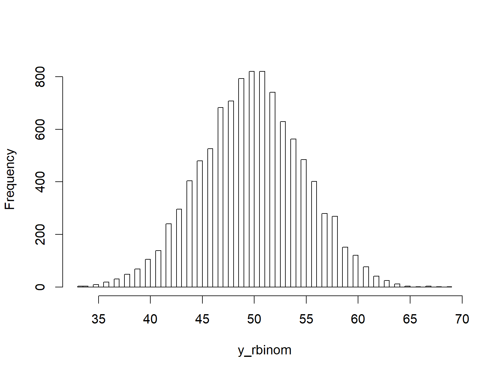
We can illustrate the distribution of our random numbers in a histogram:
hist(y_rbinom,                                        # Plot of randomly drawn binomial density
     breaks = 100,
     main = "")

Figure 4: Random Numbers Generated According to Binomial Distribution.
Note that in the previous R syntax we used a size of 100 trials and a probability of success of 0.5. In case we want to generate a random dummy variable, we simply have to set the size argument to be equal to 1:
y_rbinom_dummy <- rbinom(N, size = 1, prob = 0.5)     # Draw N dummy values
y_rbinom_dummy                                        # Print values to RStudio console
# 0 1 0 1 1 1 0 1 0 0 0 0 1 0 1 0 0 1 1 1 1 1 0 0 0 0 0 1 1 1 1 0 1 1 1...
Video, Further Resources & Summary
If you need more information on the topics of this article, you may want to have a look at the following video of my YouTube channel. I show the R programming code of this tutorial in the video:
The YouTube video will be added soon.
You could also have a look at the other posts on distributions and the generation of random numbers in R:
- Bernoulli Distribution in R
- Beta Distribution in R
- Binomial Distribution in R
- Bivariate & Multivariate Distributions in R
- Cauchy Distribution in R
- Chi-Squred Distribution in R
- Exponential Distribution in R
- F Distribution in R
- Gamma Distribution in R
- Geometric Distribution in R
- Hypergeometric Distribution in R
- Log Normal Distribution in R
- Logistic Distribution in R
- Negative Binomial Distribution in R
- Normal Distribution in R
- Poisson Distribution in R
- Student t Distribution in R
- Studentized Range Distribution in R
- Uniform Distribution in R
- Weibull Distribution in R
- Wilcoxon Signedank Statistic Distribution in R
- Wilcoxonank Sum Statistic Distribution in R
In addition, you could have a look at the related tutorials on this homepage. I have published numerous related posts already.
By the way, if you are looking for a job where the skills learned in this tutorial can be applied, you may have a look at the R programming & data science job offers on Jooble. Jooble is an ad partner of Statistics Globe and displays job offers from thousands of different sources.
In summary: In this tutorial you learned how to use the binom functions in R. Let me know in the comments below, if you have additional questions.
Subscribe to the Statistics Globe Newsletter
Get regular updates on the latest tutorials, offers & news at Statistics Globe.
I hate spam & you may opt out anytime: Privacy Policy.
Thank you!
Welcome to the Statistics Globe newsletter. From now on, I’ll send you regular emails about statistics, data science, AI, and programming with R and Python.
I’m Joachim Schork. On this website, I provide statistics tutorials as well as code in Python and R programming.
Statistics Globe Newsletter
Get regular updates on the latest tutorials, offers & news at Statistics Globe. I hate spam & you may opt out anytime: Privacy Policy.
Thank you!
Please check your email inbox and click the confirmation link to complete your subscription. If you don’t see the email within a few minutes, please also check your spam/junk folder.


