Geometric Distribution in R (4 Examples) | dgeom, pgeom, qgeom & rgeom Functions

This tutorial shows how to apply the geometric functions in the R programming language.

The tutorial contains four examples for the geom R commands. More precisely, the tutorial will consist of the following content:

• Example 1: Geometric Density in R (dgeom Function)
• Example 2: Geometric Cumulative Distribution Function (pgeom Function)
• Example 3: Geometric Quantile Function (qgeom Function)
• Example 4: Simulation of Random Numbers (rgeom Function)
• Video & Further Resources

You’re here for the answer, so let’s get straight to the examples…

Example 1: Geometric Density in R (dgeom Function)

In the first example, we will illustrate the density of the geometric distribution in a plot. As a first step, we need to create a vector of quantiles:

x_dgeom <- seq(0, 20, by = 1)                         # Specify x-values for dgeom function

Now, we can apply the dgeom function to this vector as shown in the R code below. Note that I’m using a probability of 0.5 (i.e. 50%) in the examples of this tutorial. You may modify this probability to your specific preferences.

y_dgeom <- dgeom(x_dgeom, prob = 0.5)                 # Apply dgeom function

The previous R syntax stored the density values of the geometric distribution in the data object y_dgeom. We can now plot these values with the plot R function as follows:

plot(y_dgeom)                                         # Plot dgeom values

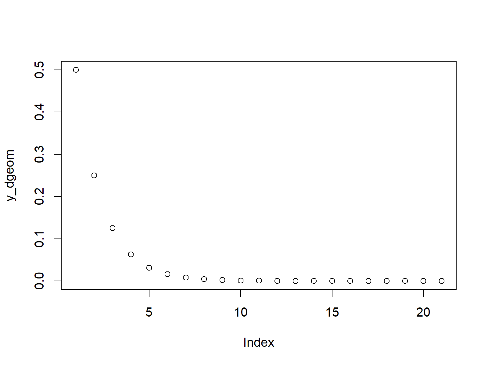
Figure 1: Application of dgeom Function.

Example 2: Geometric Cumulative Distribution Function (pgeom Function)

Example 2 shows how to draw a plot of the geometric cumulative distribution function (CDF). As in Example 1, we first need to create a sequence of quantiles:

x_pgeom <- seq(0, 20, by = 1)                         # Specify x-values for pgeom function

We can use this sequence of quantiles as input for the pgeom function:

y_pgeom <- pgeom(x_pgeom, prob = 0.5)                 # Apply pgeom function

And then, we can apply the plot function to draw a graphic containing the values of the geometric cumulative distribution function:

plot(y_pgeom)                                         # Plot pgeom values

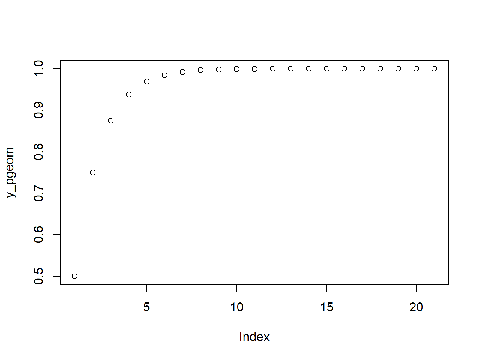
Figure 2: Application of pgeom Function.

Example 3: Geometric Quantile Function (qgeom Function)

In the third example, we will discuss the geometric quantile function. In case of the quantile function, we need to create a vector of probabilities (instead of quantiles as in Examples 1 and 2):

x_qgeom <- seq(0, 1, by = 0.01)                        # Specify x-values for qgeom function

Now, we can use the qgeom R function to return the quantile function values that correspond to our input probabilities:

y_qgeom <- qgeom(x_qgeom, prob = 0.5)                  # Apply qgeom function

Finally, we can produce a graph that is showing our quantile function values:

plot(y_qgeom)                                          # Plot qgeom values

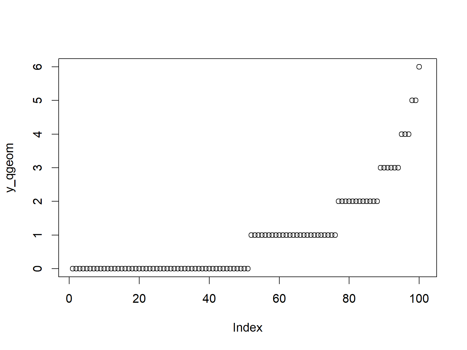
Figure 3: Application of qgeom Function.

Example 4: Simulation of Random Numbers (rgeom Function)

We can also simulate a set of random numbers, which follows the geometric distribution. For this task, we first need to specify a seed and a sample size of random numbers that we want to generate:

set.seed(53535)                                        # Set seed for reproducibility
N <- 10000                                                                # Specify sample size

Then, we can apply the rgeom function to generate our random numbers:

y_rgeom <- rgeom(N, prob = 0.5)                        # Draw N geometrically distributed values
y_rgeom                                                                   # Print values to RStudio console

The following histogram shows how our random numbers are distributed:

hist(y_rgeom,                                          # Plot of randomly drawn geom density
     breaks = 70,
     main = "")

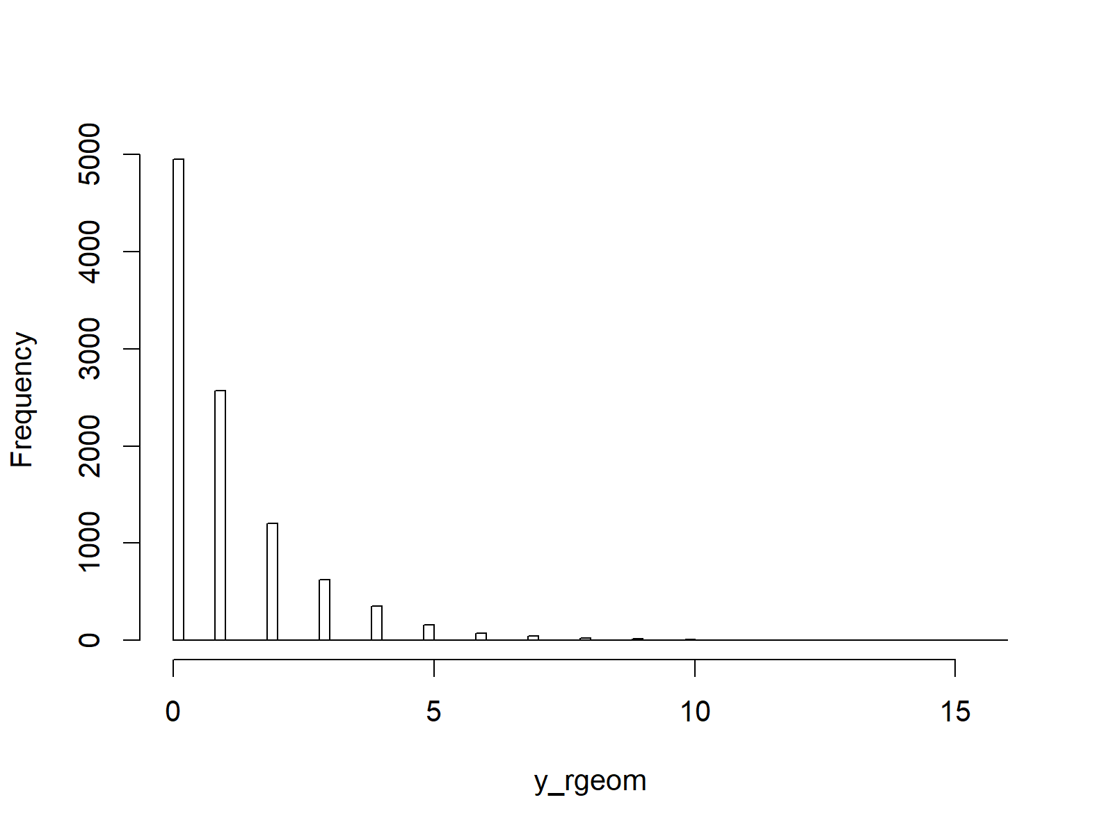
Figure 4: Application of rgeom Function.

Compare the distribution of the random numbers shown in Figure 4 and the geometric density shown in Figure 1. Both figures show the geometric distribution.

Video & Further Resources

Have a look at the following video of my YouTube channel. I’m explaining the R programming syntax of this article in the video.

The YouTube video will be added soon.

You may also have a look at the other posts on probability distributions and the simulation of random numbers in R programming:

• Bernoulli Distribution in R
• Beta Distribution in R
• Binomial Distribution in R
• Bivariate & Multivariate Distributions in R
• Cauchy Distribution in R
• Chi-Squred Distribution in R
• Exponential Distribution in R
• F Distribution in R
• Gamma Distribution in R
• Geometric Distribution in R
• Hypergeometric Distribution in R
• Log Normal Distribution in R
• Logistic Distribution in R
• Negative Binomial Distribution in R
• Normal Distribution in R
• Poisson Distribution in R
• Student t Distribution in R
• Studentized Range Distribution in R
• Uniform Distribution in R
• Weibull Distribution in R
• Wilcoxon Signedank Statistic Distribution in R
• Wilcoxonank Sum Statistic Distribution in R

In addition, you may read the other RStudio posts of my homepage. I have released several tutorials about different types of distributions already.

• R Graphics Gallery
• R Functions List (+ Examples)
• The R Programming Language

Summary: In this article you learned how to deal with the geom functions in R programming. If you have any further questions, don’t hesitate to tell me about it in the comments.