Student t distribution in R (4 Examples) | dt, pt, qt & rt Functions

This article shows how to apply the Student t functions in R.

The tutorial is structured as follows:

• Example 1: Student t Probability Density Function (dt Function)
• Example 2: Student t Cumulative Distribution Function (pt Function)
• Example 3: Student t Quantile Function (qt Function)
• Example 4: Generating Random Numbers (rt Function)
• Video, Further Resources & Summary

Let’s dive right into the examples.

Example 1: Student t Probability Density Function (dt Function)

In the first example, we’ll create a graphic showing the density of the Student t distribution.

First, we need to create a vector of quantiles in R:

x_dt <- seq(- 10, 10, by = 0.01)                    # Specify x-values for dt function

After running the previous R code, we can apply the dt command in R as follows. In the example, we use 3 degrees of freedom (as specified by the argument df = 3):

y_dt <- dt(x_dt, df = 3)                            # Apply dt function

The Student t density values are now stored in the data object y_dt. We can draw a graph representing these values with the plot R function:

plot(y_dt)                                          # Plot dt values

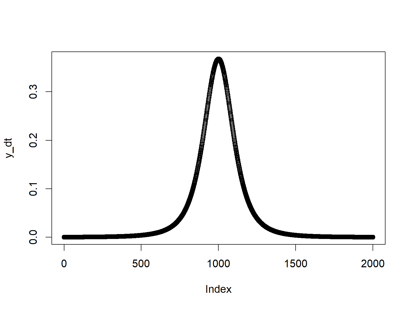
Figure 1: Density of Student t Distribution in R.

Example 2: Student t Cumulative Distribution Function (pt Function)

This example shows how to draw the cumulative distribution function (CDF) of a Student t distribution.

As in the previous example, we first need to create an input vector:

x_pt <- seq(- 10, 10, by = 0.01)                    # Specify x-values for pt function

Then, we can apply the pt function to this input vector in order to create the corresponding CDF values:

y_pt <- pt(x_pt, df = 3)                            # Apply pt function

Finally, we can apply the plot function to draw a graphic representing the CDF of the Student t distribution in R:

plot(y_pt)                                          # Plot pt values

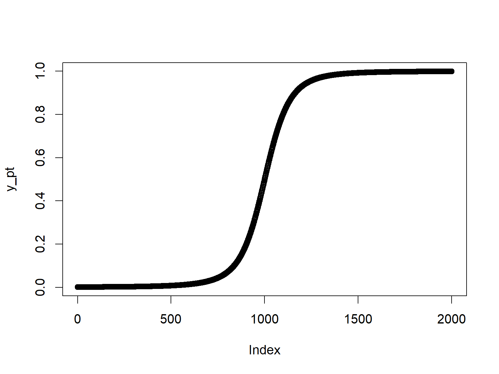
Figure 2: Cumulative Distribution Function of Student t Distribution in R.

Example 3: Student t Quantile Function (qt Function)

If we want to draw a plot of the quantile function of the Student t distribution, we need to create a sequence of probabilities as input:

x_qt <- seq(0, 1, by = 0.01)                        # Specify x-values for qt function

We then can apply the qt R command to these probabilities:

y_qt <- qt(x_qt, df = 3)                            # Apply qt function

The corresponding plot can be created with the plot function as follows:

plot(y_qt)                                          # Plot qt values

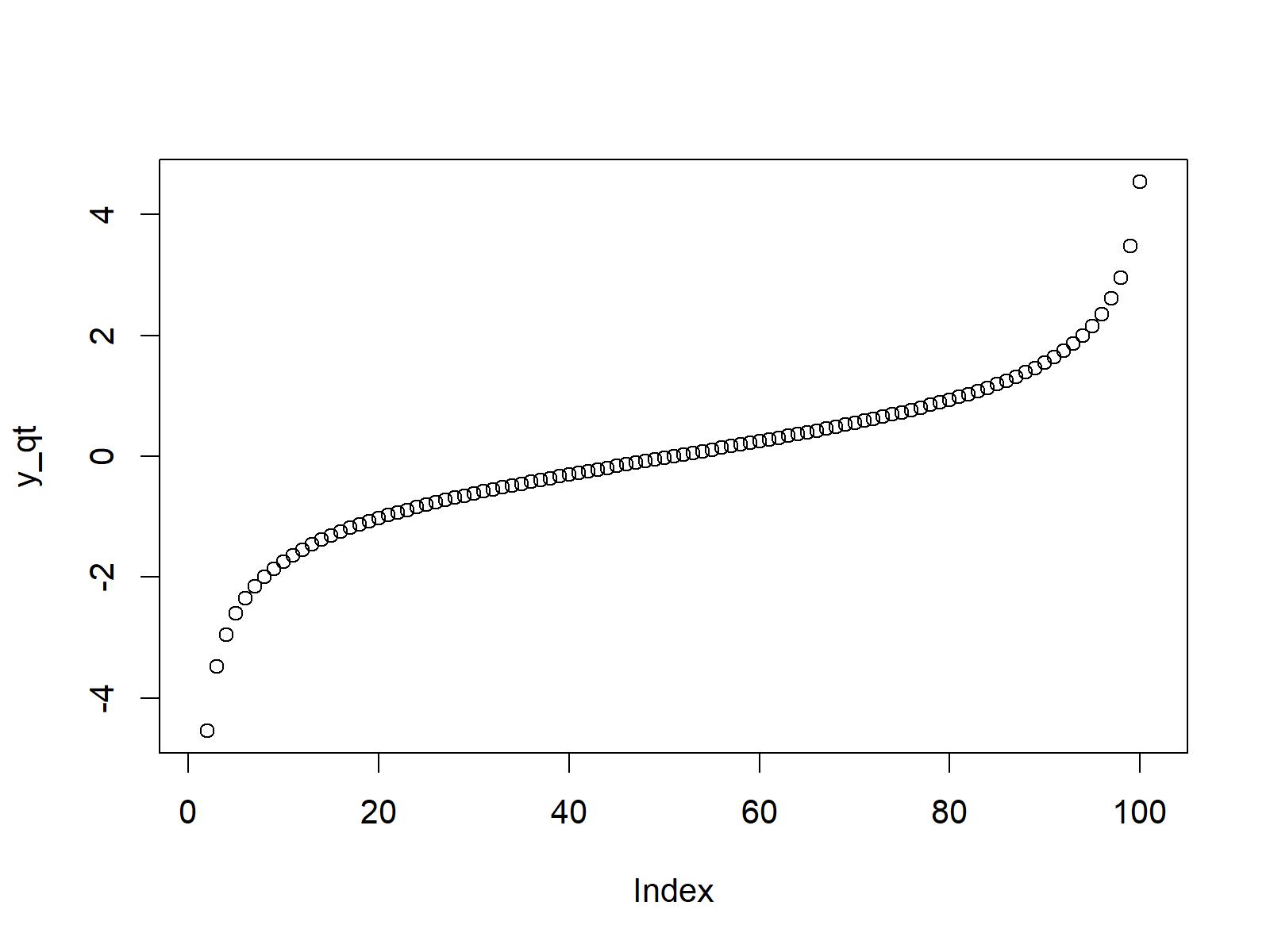
Figure 3: Quantile Function of Student t Distribution in R.

Example 4: Generating Random Numbers (rt Function)

We can also apply the Student t functions in order to generate random numbers. First, we have to set a seed for reproducibility and we also need to specify a sample size N that we want to simulate:

set.seed(91929)                                     # Set seed for reproducibility
N <- 10000                                          # Specify sample size

We can now use the rt function to generate our set of random numbers:

y_rt <- rt(N, df = 3)                               # Draw N log normally distributed values
y_rt                                                # Print values to RStudio console

The following histogram illustrates the distribution of our random numbers (i.e. a Student t distribution):

hist(y_rt,                                          # Plot of randomly drawn student t density
     breaks = 100,
     main = "")

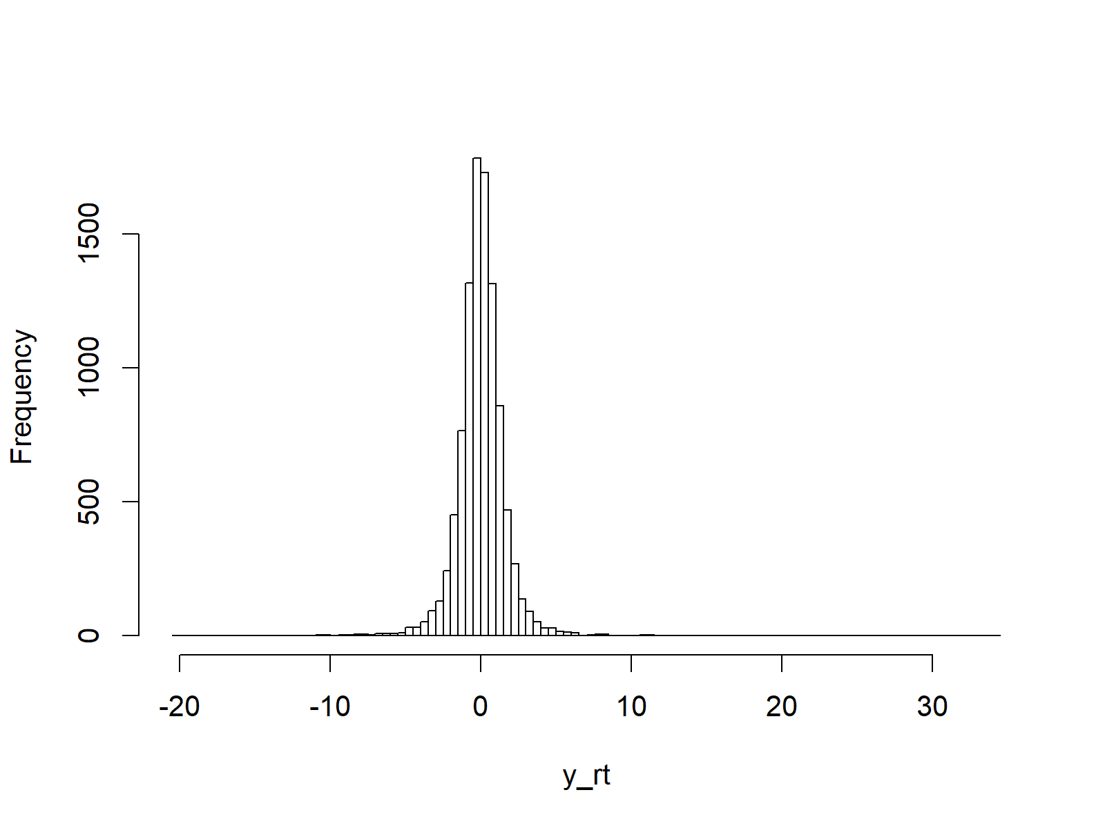
Figure 4: Random Numbers According to Student t Distribution in R.

Video, Further Resources & Summary

Have a look at the following video of my YouTube channel. In the video tutorial, I’m explaining the contents of this tutorial.

The YouTube video will be added soon.

You may also have a look at the other articles on distributions and the simulation of random numbers in R:

• Bernoulli Distribution in R
• Beta Distribution in R
• Binomial Distribution in R
• Bivariate & Multivariate Distributions in R
• Cauchy Distribution in R
• Chi-Squred Distribution in R
• Exponential Distribution in R
• F Distribution in R
• Gamma Distribution in R
• Geometric Distribution in R
• Hypergeometric Distribution in R
• Log Normal Distribution in R
• Logistic Distribution in R
• Negative Binomial Distribution in R
• Normal Distribution in R
• Poisson Distribution in R
• Student t Distribution in R
• Studentized Range Distribution in R
• Uniform Distribution in R
• Weibull Distribution in R
• Wilcoxon Signedank Statistic Distribution in R
• Wilcoxonank Sum Statistic Distribution in R

Furthermore, I can recommend to read the related tutorials on this website. Please find a selection of interesting articles here.

• R Graphics Gallery
• R Functions List (+ Examples)
• The R Programming Language

In this article you learned how to draw and simulate a Student t distribution in the R programming language. Please let me know in the comments below, in case you have any further questions.