data.table Package in R | Tutorial & Programming Examples
The R package data.table was created as an improved version of the base R data.frame. It comes with increased speed, efficiently written functions, and has a nice, easy-to-understand syntax, as we will see in the following examples. It allows for fast and easy data manipulation, especially for large datasets.
In this article, I’ll demonstrate how to get started with the data.table package in R. This introduction is based on the data.table github page and the CRAN post on data.table. Furthermore, there is the CRAN documentation and CRAN page on the package for more information.
The article consists of six examples in which we demonstrate the features of the data.table package. More precisely, the post is structured as follows:
Let’s dive right into the exemplifying R code!
Example Data & Packages
First, we have to install and load the data.table software package:
install.packages("data.table")                           # Install & load data.table
library("data.table")
We start right away by generating a data.table in R. For the generation of data.tables, we also recommend you to take a look at our blog posts: create data.table, create empty data.table, and convert data.frame or matrix into data.table.
N <- 100000                                              # Number of observations
set.seed(6)                                              # Set seed for reproducible results
DT_1 <- data.table( "A" = rnorm(N),                      # Create a data.table
                    "B" = rpois(N, 5),
                    "C" = sample(c(TRUE, FALSE),       N, replace = TRUE),
                    "D" = factor(sample(letters[1:20], N, replace = TRUE)),
                    "E" = sample(month.abb[1:12],      N, replace = TRUE) )
You can see that we created the data in data.table DT_1 with random samples from chosen categories, click here if you want to get more information regarding the sample function. Let us take a look at the data.
head(DT_1) # Print the head of the data
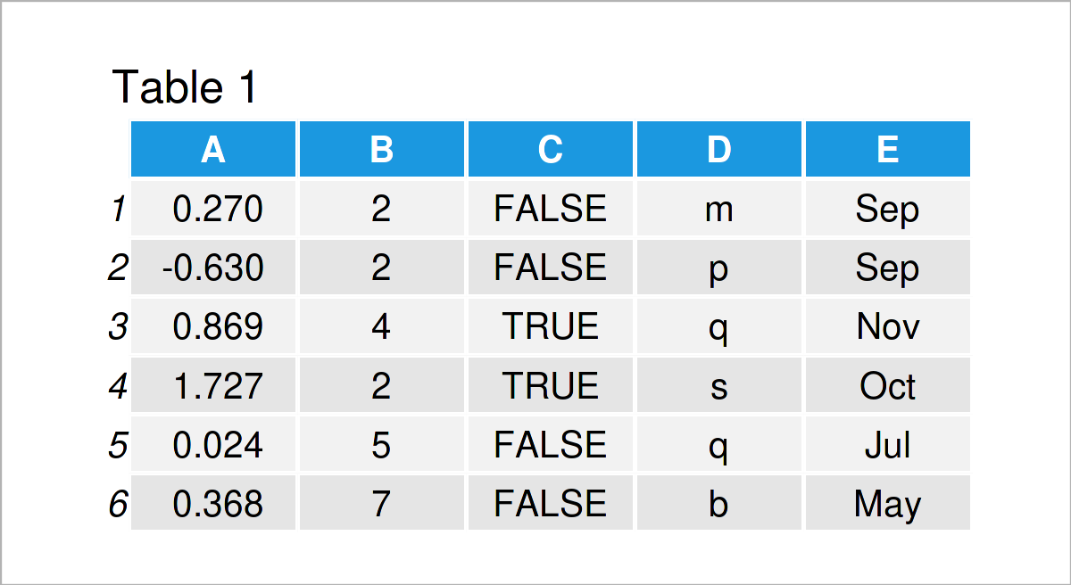
Table 1 shows that we just created a data.table, which consists of 100000 observations of five variables with different types. For more information on the data, we can also take a look at the structure of the data with function str().
str(DT_1)                                                # Display the structure of the data
# Classes ‘data.table’ and 'data.frame':	100000 obs. of  5 variables:
#  $ A: num  0.2696 -0.63 0.8687 1.7272 0.0242 ...
#  $ B: int  2 2 4 2 5 7 3 5 4 6 ...
#  $ C: logi  FALSE FALSE TRUE TRUE FALSE FALSE ...
#  $ D: Factor w/ 20 levels "a","b","c","d",..: 13 16 17 19 17 2 3 20 7 14 ...
#  $ E: chr  "Sep" "Sep" "Nov" "Oct" ...
#  - attr(*, ".internal.selfref")=<externalptr>
We see that the class of the data is data.table and data.frame. If you are familiar with data.frames in R, you probably already noticed the similarity between the two. With the data creation and structure, we can see that data.table builds on data.frames in R.
Example 1: Select a Single Column
In Example 1, I’ll demonstrate how to address a single column of a data.table. As with a data.frame, we can use the ‘$’ sign and the name of the column which we want to address. Then, the column is returned as a vector.
head(DT_1$A)                                               # Possibility 1
# [1]  0.26960598 -0.62998541  0.86865983  1.72719552  0.02418764  0.36802518
We get the same results with the following code.
head(DT_1[, A])                                             # Possibility 2
# [1]  0.26960598 -0.62998541  0.86865983  1.72719552  0.02418764  0.36802518
This time we used brackets ‘[ , ]’. However, other than with data.frames, in data.tables we can skip the quotation marks around the column names.
Alternatively, we can index the number of the respective column, similar to a data.frame. The first column is selected as ‘[ , 1]’. This way (and this is different from a data.frame), however, the result itself is a data.table with only one column.
head(DT_1[, 1]) # Possibility 3
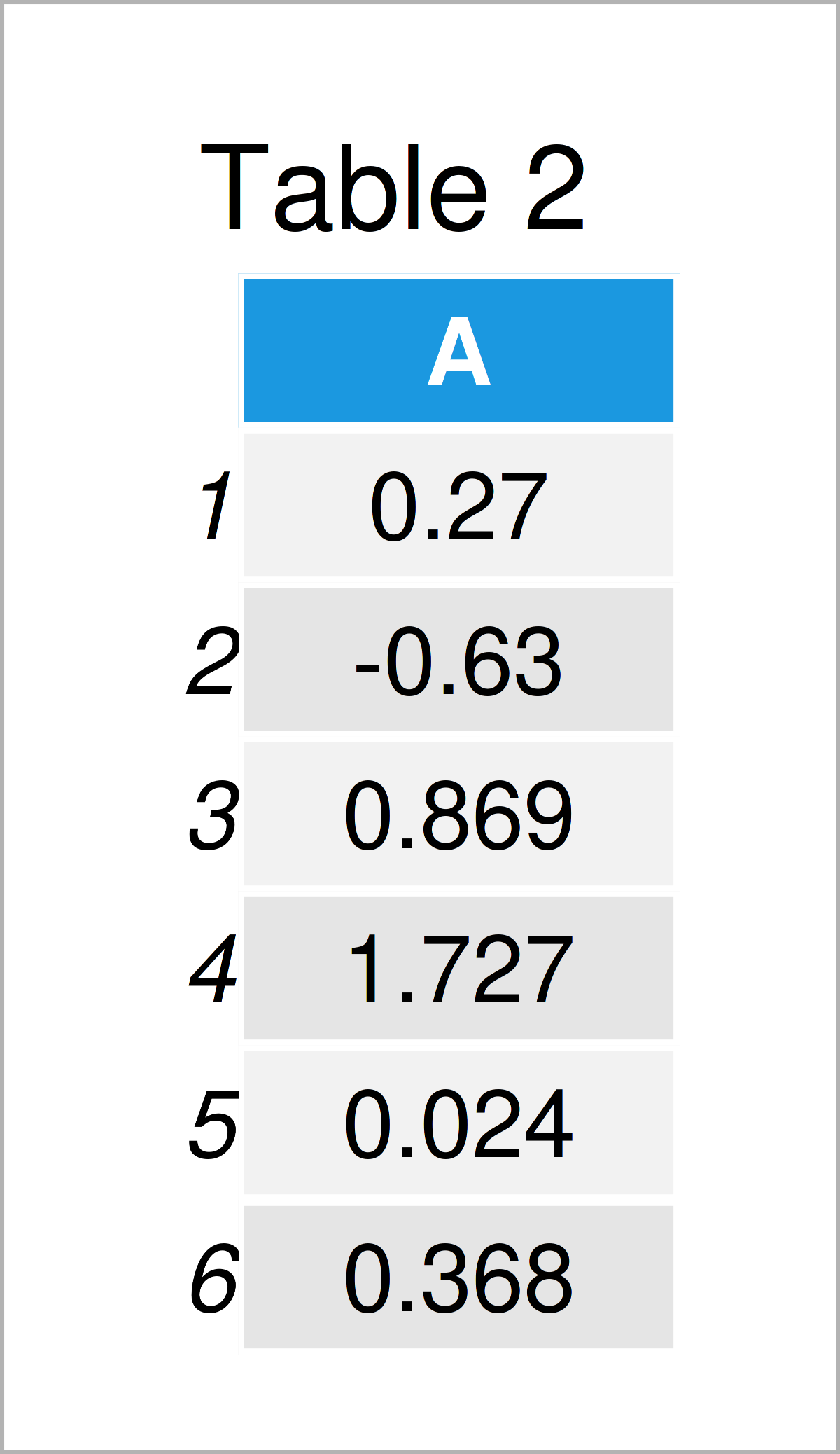
As revealed in Table 2, the previous R code has created a data.table with only one column.
When the names of the columns which you want to address are stored as characters in another object, the following way of addressing specific columns comes in handy.
column_to_choose <- "A"
head(DT_1[, .SD, .SDcols = column_to_choose])               # Possibility 4

The output of the previous R syntax is shown in Table 3 – The selection of a single column again returns a data.table object. You can also use ‘.SDcols’ to choose several columns at once.
Example 2: Subset the Data
In this example, I’ll explain how to subset a data.table within brackets in the way ‘[ chosen rows , chosen columns ]’. Like in a data.frame, we can for example use ‘[ 1:10, ]’ to select the first 10 rows of a data.table.
The following example code shows a slightly more advanced subsetting.
DT_2 <- DT_1[ C == TRUE & E %in% month.abb[1:6], ]       # Data subset
head(DT_2)                                               # Print head of the data
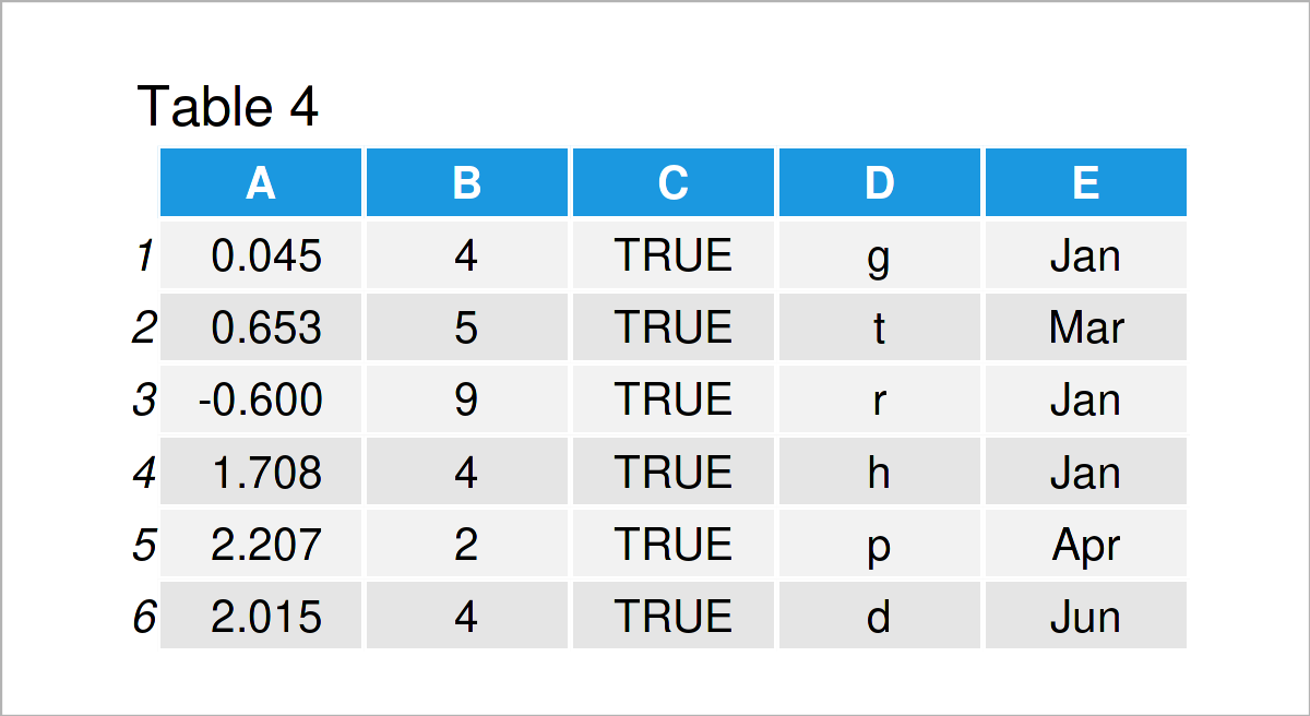
As shown in Table 4, the previous R code has created a data.table which contains only those rows of DT_1 in which column C is equal to TRUE and column E is equal to the first six months of a year. With this example you can see how easy the syntax of data.tables is to read and write compared to the syntax of a data.frame.
Example 3: Calculate Statistics for Data Subsets
Example 3 demonstrates how to select a subset of a data.table and calculate statistics based on this subset, all within the brackets ‘[ , ]’. With this example you might also see a similarity of the syntax to that of SQL, as is also demonstrated here.
DT_1[ C == TRUE & D %in% letters[1:10], summary(A + B)]  # Calculate summary statistics
#    Min. 1st Qu.  Median    Mean 3rd Qu.    Max.
#  -3.237   3.255   4.844   5.000   6.590  18.931
With the above example, we calculated the summary statistics of the sum of variables A and B for all those rows of DT_1 for which variable C is true and variable D takes letters one to ten. From this example, you can see that very little code is needed in the data.table syntax to perform more complicated functions. Also, no nested bracketing is necessary.
Example 4: Calculate Statistics by Data Groups
In this example, I’ll demonstrate how to calculate statistics for certain groups in a data.table. For that, not that the third entry within brackets ‘[ , , ]’ can be used for grouping arguments.
DT_1[ E %in% month.abb[1:6], list("mean_A" = mean(A), "sum_A" = sum(A)), by = E]
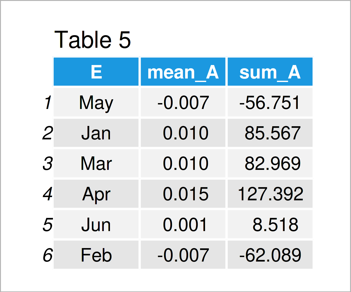
In Table 5 you can see that with the previous R code we created a data.table which holds the mean and sum of variable A for each unique value of variable E, calculated for those rows of DT_1 in which variable E is equal to the first six months.
Example 5: Count Number of Rows for Which Certain Conditions Hold
Example 5 explains how to count the number of rows in a data.table. With the following code, we calculate the number of data rows of DT_1 for which variable C is true, variable D takes letters one to ten, and variable E takes the first six months.
DT_1[ C == TRUE & D %in% letters[1:10] & E %in% month.abb[1:6], .N]
# [1] 12486
Next, we create a new column called N using ‘N := ‘. We define N as the number of rows for which C is false for the cross-combinations of variables D and E.
DT_3 <- data.table::copy(DT_1)                           # Replicate the data
DT_4 <- DT_3[ C == FALSE, "N" := .N, by = list(D, E)]
head(DT_4)
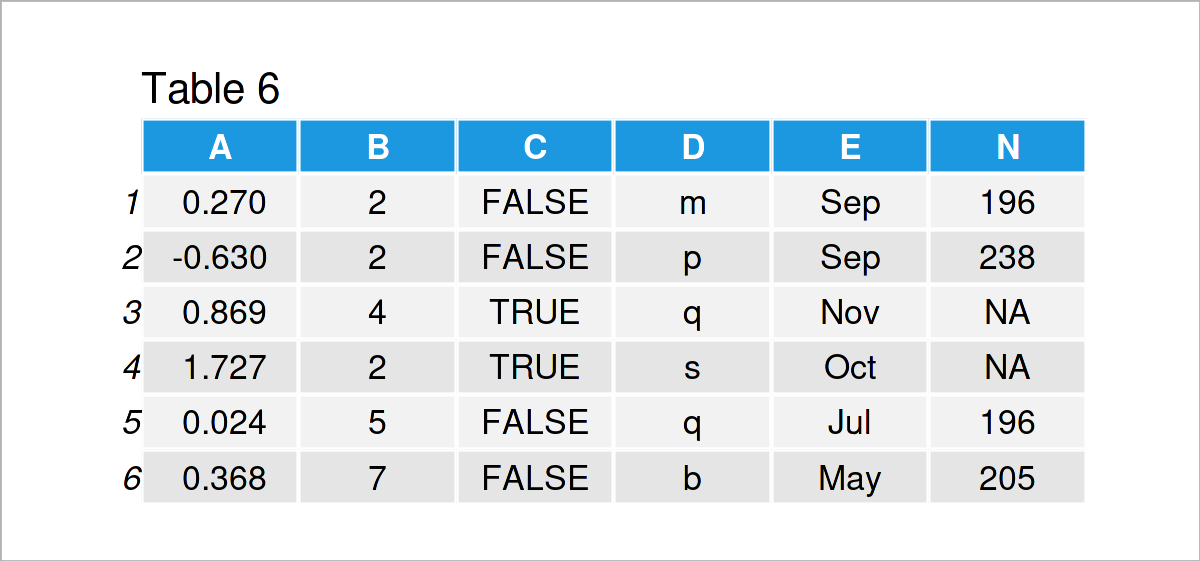
The output of the previous R programming syntax is shown in Table 6 – We see that (for all rows with C equal to false), there are 196 rows in which D=m and E=Sep. Equivalently, there are 238 rows in which D=p and E=Sep and there is no row with D=q and E=Nov.
Example 6: Create Plots For data.table Subsets
And there is much more to do with data.tables! In Example 6, I’ll illustrate how to create plots directly from the data.table brackets ‘[ , ]’. We first create a new column mean_A which holds the mean value of A for the cross-combinations of variables C, D, and E. In the next step, we plot the first 100 values of mean_A and B.
DT_5 <- DT_1[ , "mean_A" := mean(A), by = list(C, D, E)]
DT_5[ 1:100, plot(mean_A, B, pch = 20, col = "blue") ]
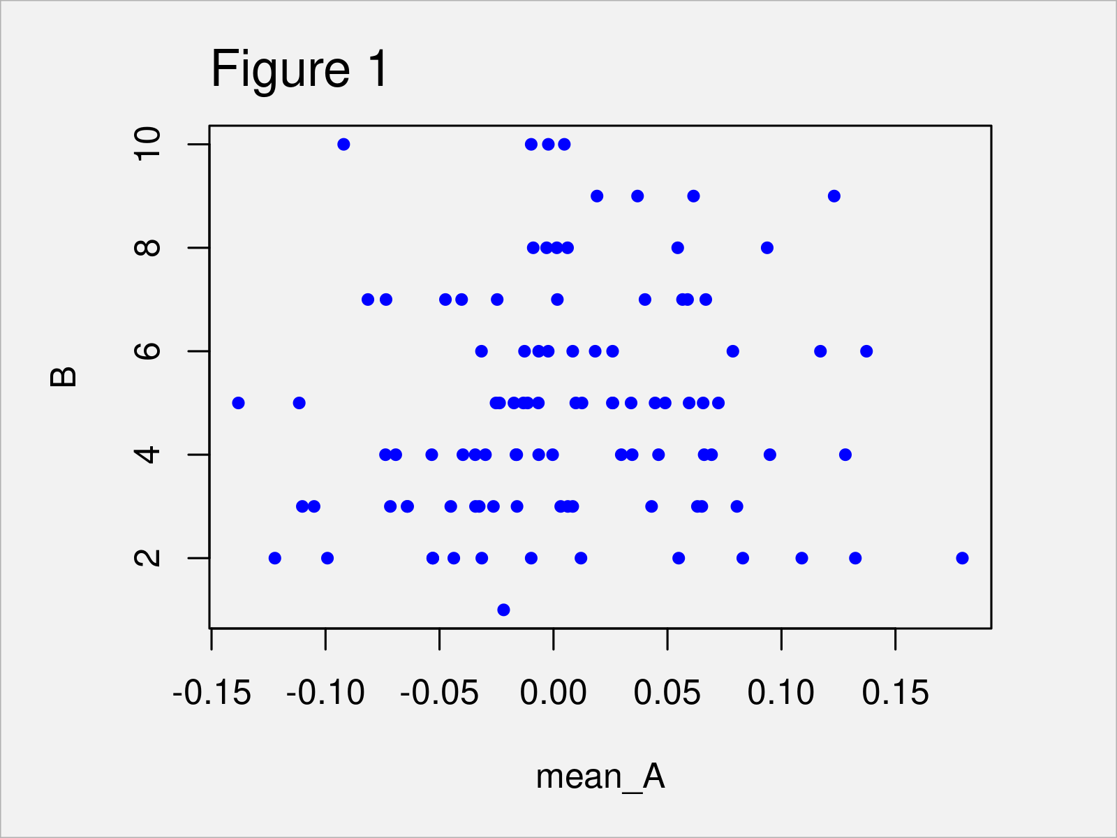
After executing the previous R programming code the scatterplot in Figure 1 has been created.
Further Tutorials on the data.table Package
You can find tutorials and examples for the data.table package below.
Other Useful R Packages
In the following, you can find a list of other useful R packages.
This page was created in collaboration with Anna-Lena Wölwer. Have a look at Anna-Lena’s author page to get further details about her academic background and the other articles she has written for Statistics Globe.





















2 Comments. Leave new
hi i look at all your video related to month and i still couldn’t find the answer i was looking for. So, i was wondering if you can make a video that DOES NOT DEAL WITH DATE and show how one can graph the months in Calander order. ex X <- c(feb, jan, feb, jul, feb, dec, feb, may,feb). how do i graph X so that does month shows "jan, feb, may, jul, and dec" and NOT "dec, feb, jan, jul, and may"
thank you
Hey,
You may order your plot manually as shown in this tutorial.
I hope that helps!
Joachim