Principal Component Analysis (PCA) in R

In this tutorial you’ll learn how to perform a Principal Component Analysis (PCA) in R.

The table of content is structured as follows:

This page was created in collaboration with Paula Villasante Soriano and Cansu Kebabci. Please have a look at Paula’s and Cansu’s author pages to get further information about their academic backgrounds and the other articles they have written for Statistics Globe.

 
Let’s take a look at the procedure in R!
 

Example Data & Add-On Packages

In this tutorial, we will use the biopsy data of the MASS package. This is a breast cancer database obtained from the University of Wisconsin Hospitals, Dr. William H. Wolberg. He assessed biopsies of breast tumors for 699 patients.

In order to use this database, we need to install the MASS package first, as follows.

install.packages("MASS")

In order to visualize our data, we will install the factoextra and ggplot2 packages.

install.packages("factoextra")
install.packages("ggplot2")

Next, we will load the libraries.

library(MASS)
library(factoextra)
library(ggplot2)

Now, we can import the biopsy data and print a summary via str().

data(biopsy)
str(biopsy)
 
#'data.frame':	699 obs. of  11 variables:
# $ ID   : chr  "1000025" "1002945" "1015425" "1016277" ...
# $ V1   : int  5 5 3 6 4 8 1 2 2 4 ...
# $ V2   : int  1 4 1 8 1 10 1 1 1 2 ...
# $ V3   : int  1 4 1 8 1 10 1 2 1 1 ...
# $ V4   : int  1 5 1 1 3 8 1 1 1 1 ...
# $ V5   : int  2 7 2 3 2 7 2 2 2 2 ...
# $ V6   : int  1 10 2 4 1 10 10 1 1 1 ...
# $ V7   : int  3 3 3 3 3 9 3 3 1 2 ...
# $ V8   : int  1 2 1 7 1 7 1 1 1 1 ...
# $ V9   : int  1 1 1 1 1 1 1 1 5 1 ...
# $ class: Factor w/ 2 levels "benign",
# "malignant": 1 1 1 1 1 2 1 1 1 1 ...

As shown below, the biopsy data contains 699 observations of 11 variables. The output also shows that there’s a character variable: ID, and a factor variable: class, with two levels: benign and malignant.

We will exclude the non-numerical variables before conducting the PCA, as PCA is mainly compatible with numerical data with some exceptions. We will also exclude the observations with missing values using the na.omit() function to keep it simple. For other alternatives, see missing data imputation techniques.

data_biopsy <- na.omit(biopsy[,-c(1,11)])

Now, we’re ready to conduct the analysis!

Step 1: Calculate Principal Components

The first step is to calculate the principal components. To accomplish this, we will use the prcomp() function, see below.

biopsy_pca <- prcomp(data_biopsy, 
                     scale = TRUE)

The “scale = TRUE” argument allows us to make sure that each variable in the biopsy data is scaled to have a mean of 0 and a standard deviation of 1 before calculating the principal components. To see the difference between analyzing with and without standardization, see PCA Using Correlation & Covariance Matrix.

Let’s check the elements of our biopsy_pca object!

names(biopsy_pca)
 
# [1] "sdev"     "rotation" "center"   "scale"    "x"

The "sdev" element corresponds to the standard deviation of the principal components; the "rotation" element shows the weights (eigenvectors) that are used in the linear transformation to the principal components; "center" and "scale" refer to the means and standard deviations of the original variables before the transformation; lastly, "x" stores the principal component scores. All can be called via the $ operator.

Let’s now see the summary of the analysis using the summary() function!

summary(biopsy_pca)
 
# Importance of components:
#                          PC1     PC2     PC3     PC4     PC5     PC6     PC7     PC8     PC9
# Standard deviation     2.4289 0.88088 0.73434 0.67796 0.61667 0.54943 0.54259 0.51062 0.29729
# Proportion of Variance 0.6555 0.08622 0.05992 0.05107 0.04225 0.03354 0.03271 0.02897 0.00982
# Cumulative Proportion  0.6555 0.74172 0.80163 0.85270 0.89496 0.92850 0.96121 0.99018 1.00000

The first row gives the standard deviation of each component, which can also be retrieved via biopsy_pca$sdev. The second row shows the percentage of explained variance, also obtained as follows.

biopsy_pca$sdev^2 / sum(biopsy_pca$sdev^2)
 
# [1] 0.655499928 0.086216321 0.059916916 0.051069717 0.042252870
# [6] 0.033541828 0.032711413 0.028970651 0.009820358

Accordingly, the first principal component explains around 65% of the total variance, the second principal component explains about 9% of the variance, and this goes further down with each component. Please be aware that biopsy_pca$sdev^2 corresponds to the eigenvalues of the principal components.

Finally, the last row, Cumulative Proportion, calculates the cumulative sum of the second row. By all, we are done with the computation of PCA in R. Now, it is time to decide the number of components to retain based on there obtained results.

Step 2: Ideal Number of Components

There are several ways to decide on the number of components to retain; see our tutorial: Choose Optimal Number of Components for PCA. As one alternative, we will visualize the percentage of explained variance per principal component by using a scree plot. We will call the fviz_eig() function of the factoextra package for the application.

fviz_eig(biopsy_pca, 
         addlabels = TRUE, 
         ylim = c(0, 70))

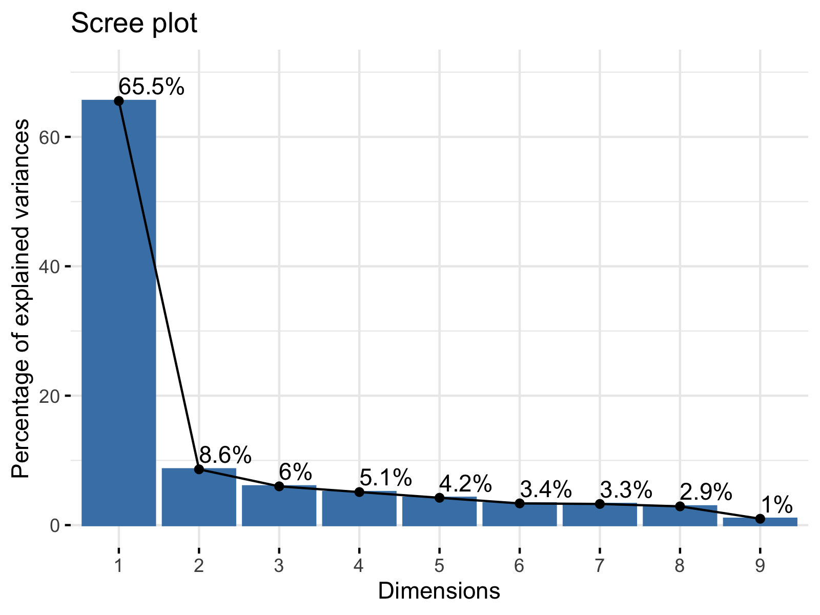
As seen, the scree plot simply visualizes the output of summary(biopsy_pca). In order to learn how to interpret the result, you can visit our Scree Plot Explained tutorial and see Scree Plot in R to implement it in R.

Step 3: Interpret Results

Visualization is essential in the interpretation of PCA results. Based on the number of retained principal components, which is usually the first few, the observations expressed in component scores can be plotted in several ways. Please see our Visualisation of PCA in R tutorial to find the best application for your purpose.

In PCA, maybe the most common and useful plots to understand the results are biplots. In this tutorial, we will use the fviz_pca_biplot() function of the factoextra package. We will also use the label="var" argument to label the variables. See the related code below.

fviz_pca_biplot(biopsy_pca,
                label="var")

Let’s see the output!

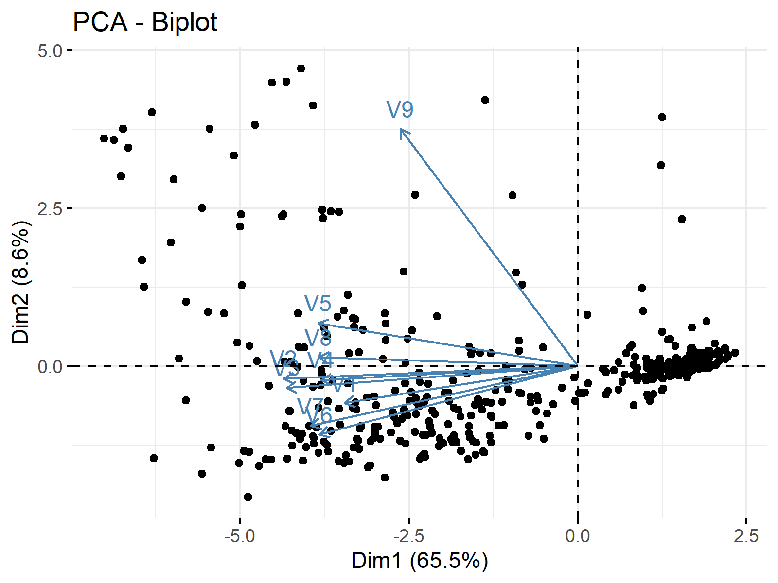
By default, the principal components are labeled Dim1 and Dim2 on the axes with the explained variance information in the parenthesis. As the ggplot2 package is a dependency of factoextra, the user can use the same methods used in ggplot2, e.g., relabeling the axes, for the visual manipulations.

For other alternatives, we suggest you see the tutorial: Biplot in R and if you wonder how you should interpret a visual like this, please see Biplots Explained.

Video, Further Resources & Summary

Do you need more explanations on how to perform a PCA in R? Then you should have a look at the following YouTube video of the Statistics Globe YouTube channel.

Furthermore, you could have a look at some of the other tutorials on Statistics Globe:

• Principal Component Analysis (PCA) Explained
• Choose Optimal Number of Components for PCA
• Scree Plot for PCA Explained
• Biplot of PCA in R
• Can PCA be Used for Categorical Variables?
• PCA Using Correlation & Covariance Matrix

This post has shown how to perform a PCA in R. In case you have further questions, you may leave a comment below.