Choose Optimal Number of Components for PCA (Theory & Example)

In this tutorial, you’ll learn how to choose the optimal number of components in a Principal Component Analysis (PCA). We’ll explain theoretically why a certain number of components is enough to keep and how to decide on the exact number.

The table of content is structured as follows:

This page was created in collaboration with Paula Villasante Soriano and Cansu Kebabci. Please have a look at Paula’s and Cansu’s author pages to get further information about their academic backgrounds and the other articles they have written for Statistics Globe.

Let’s take a look!

Sample Data

For illustration, we will use the mtcars dataset to perform a PCA. Let’s have a quick look at what the first few rows of data look like. As seen in Table 1, the dataset contains 11 numerical variables showing the features of each car model.

Now we can conduct a PCA to explain the data variation in a more compact and interpretable way. If you want to learn more about what PCA does and when and why to use it see our extensive tutorial: PCA Explained. If you wonder how to conduct the analysis in R or Python, see our tutorials: How to Use PCA in R and How to Use PCA in Python.

Before getting started, let’s explain what the principal components exactly are.

Principal Components

Principal components are the linear transformations of the original variables in the dataset. The components can be created as many as the number of original variables. However, the ones which account for most of the data variation are retained in the analysis while the rest is omitted. As a result, the data can be described by fewer features than the original, which will ease the statistical inference.

How to Choose Principal Components

No general method works in every situation for choosing the optimal number of principal components. It depends on the reason behind conducting the PCA and the priorities of the user. Let’s see what our alternatives are!

1. You Want to Visualize the Data

If you intend to visualize your data in a more interpretable way, you can conduct a PCA and select the first two or three principal components for the visualization. Choosing two principal components would lead to a two-dimensional plot (e.g., scatter plot) and choosing three principal components would lead to a three-dimensional plot. For further information on possible PCA visualizations, see our tutorials: Visualization of PCA in R and Visualization of PCA in Python.

2. You Want to Reduce the Number of Variables

You have different possibilities if the aim is to reduce the number of features in the dataset. Let’s take a look!

2.1. Setting Threshold for Explained Variance

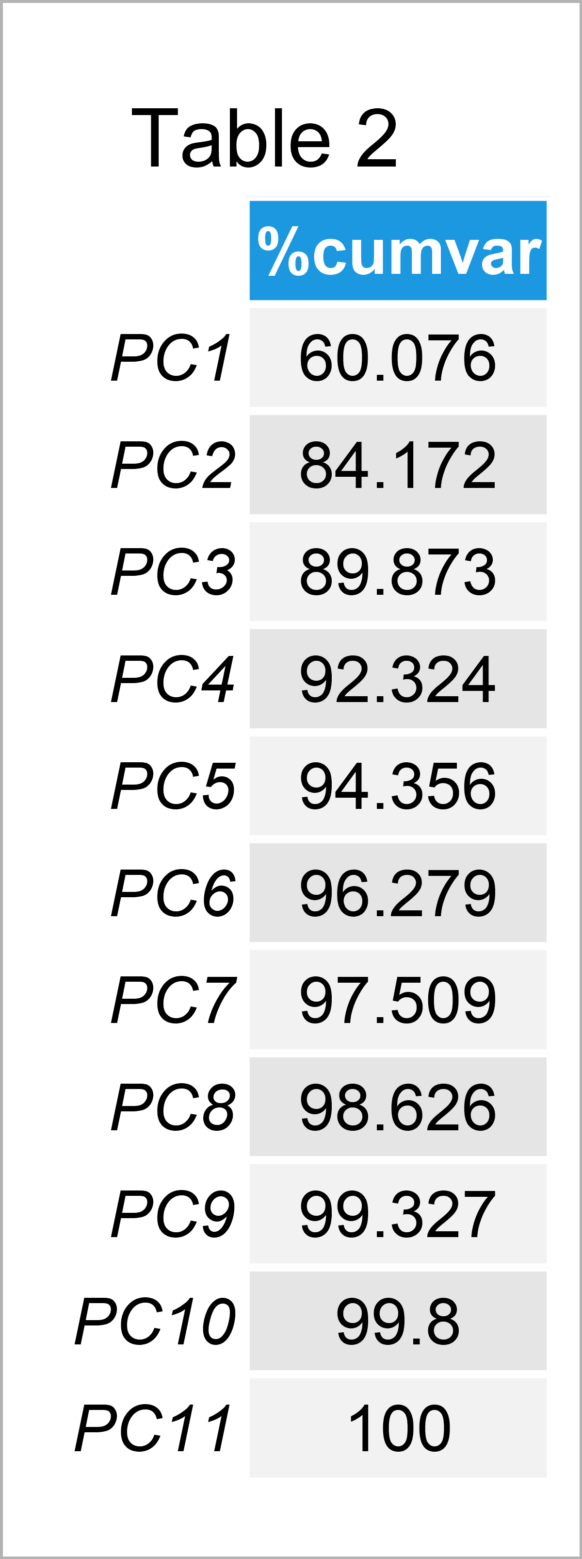
If the user wants at least a certain amount of variance to be explained, she can set a threshold in advance. For instance, if it is 80%, the principal components which account for 80% of the cumulative variance should be selected. In our case, the cumulative explained variances per component are like in Table 2. To learn how to extract the explained variance in Python and R, see our tutorials: How to Use PCA in R and How to Use PCA in Python.

As seen in Table 2, the first two principal components explain more than 80% of the total variance in the dataset. Therefore, the first two components are adequate to use for statistical inference.

Be aware that in the use of all components, the total variability in the dataset would be accounted for; see that the principal component PC11 has 100% of cumulative variance. However, there is no point in using the principal components in replacement with the original variables in such a case, as the redundant information inherited by the original variables would be kept.

This is a rather subjective method of selecting principal components; thus, this may not be the most effective way to remove redundancy. Let’s see what else we can use!

2.2. Using Kaiser’s Rule

According to Kaiser’s rule, all the components with eigenvalues greater than 1 should be kept for statistical inference. The reasoning behind Kaiser’s rule is that any principal component retained should explain the variance at least as much as an original standardized variable. Visit our tutorial What is PCA? to understand the relation between the eigenvalues and the variance in standardized PCA.

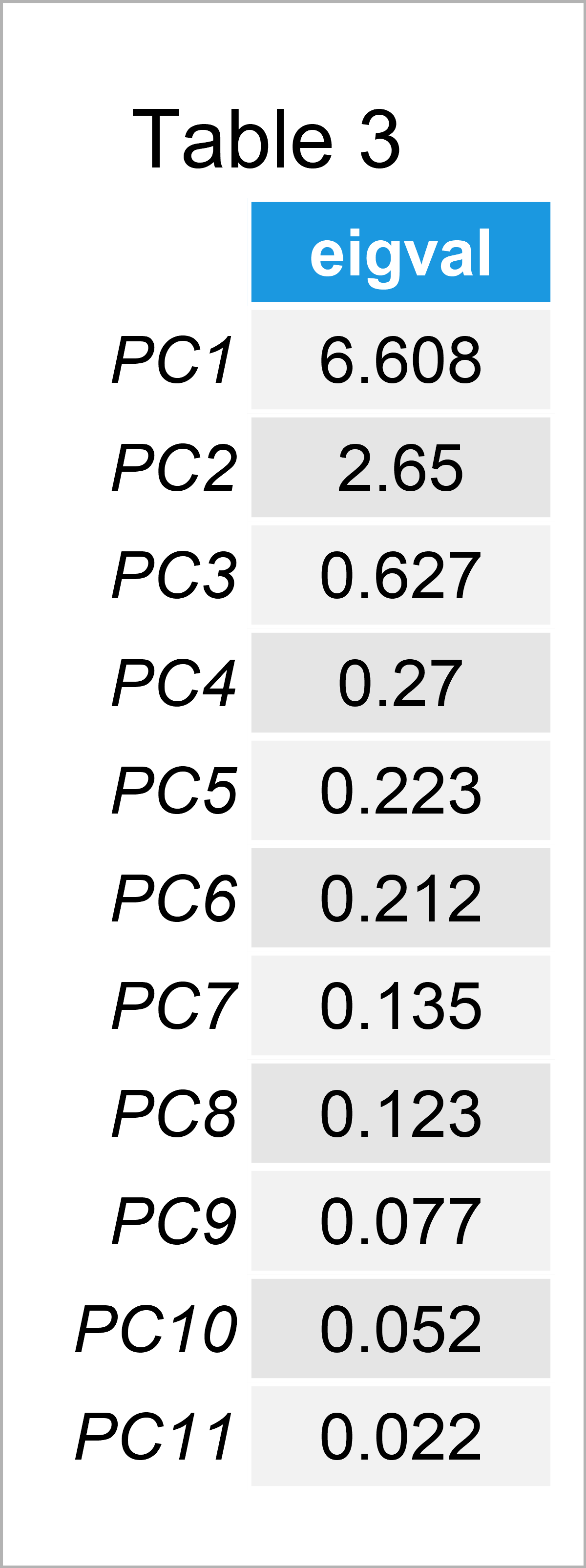
Let’s observe the eigenvalues per principal component given in Table 3 and decide which components to keep! To learn how to extract the eigenvalues in R and Python, see the Apply PCA in R and Apply PCA in Python tutorials.

According to Table 3, the eigenvalues of PC1 and PC2 are greater than 1, so we should keep the first two principal components for the statistical interpretation.

2.3. Plotting Scree Plot

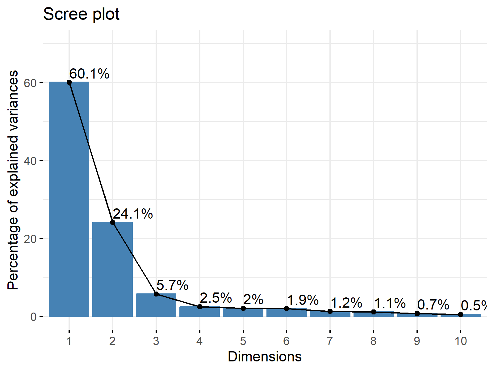
Another way of deciding on the relevant components is to visualize the explained variance per principal component. The special plots helping this visualization are called scree plots; see Figure 1 below. If you want to learn how to plot a scree plot in R and Python, see our tutorials Scree Plot of PCA in R and Scree Plot of PCA in Python.

The point where a substantial drop occurs in the graph is called elbow. According to the rule, the components appearing after the elbow are omitted. Thus, the components with relatively high explained variances are kept.

Let’s check Figure 1 to inspect the components to be retained!

Based on the scree plot above, the elbow appears at the third component; hence the first three components should be held to derive conclusions. Alternatively, Kaiser’s rule and the scree plot approach can be combined; see the Scree Plot for PCA Explained tutorial.

2.3. Using Permutation Test

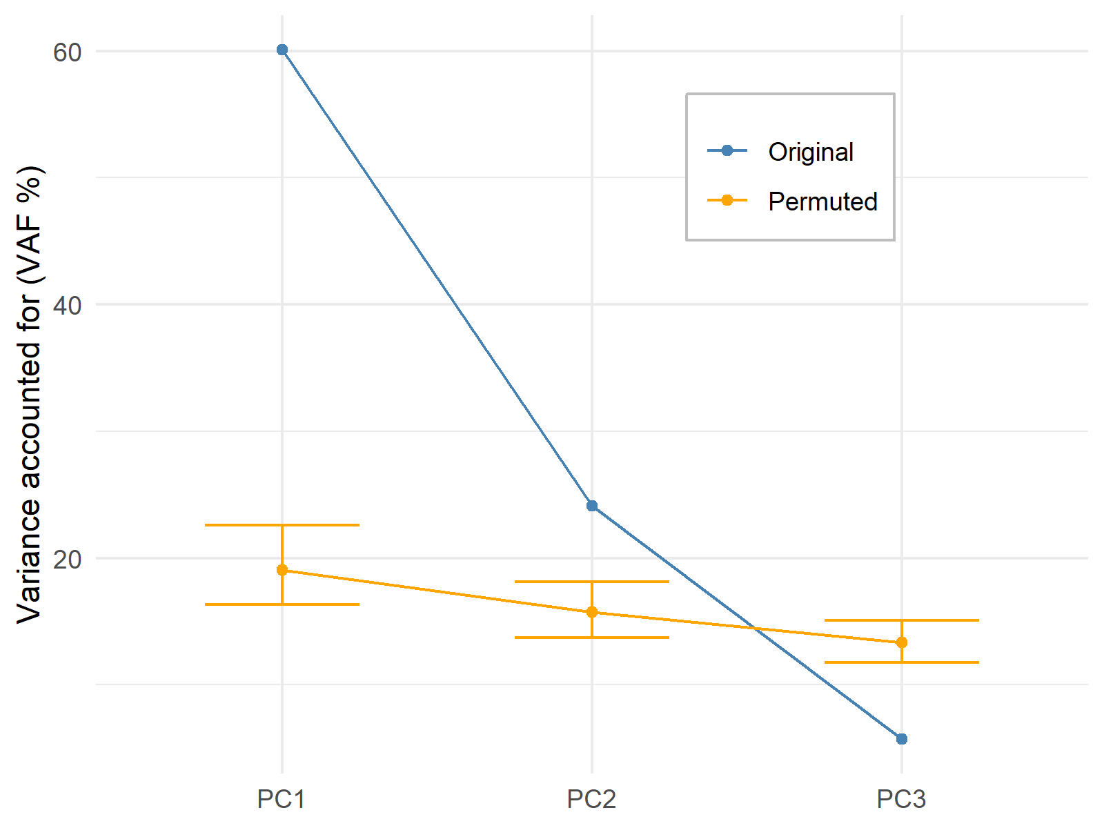
The permutation test, also called the randomization test, is another technique to decide on the number of components to retain in the analysis. The basic idea behind the test is to compare the explained variances in the original PCA with the explained variances in the PCAs rerunning on the dataset after several data permutations.

The higher the number of times an original principal component accounts for more variance than a principal component computed after a permutation, the more evidence that the particular component should be kept.

The number of comparisons, hence the number of permutations, is up to the user. For demonstration, the data is 1000 times permuted and the first three principal components are compared.

The test hypothesizes that the explained variance by the original components and the components of the re-running PCAs are more or less the same. Thus, the significant p-values indicate that there is enough evidence that the principal component explains more variance than the principal components computed based on the permuted datasets.

This graphic shows that the p-values for the first two principal components give significant results; hence the first two components should remain in the analysis.

 
As shown, there are multiple ways to choose the optimal number of components in PCA. It’s important to check different methods and select the one which gives the best result for the specific case at hand.

Video, Further Resources & Summary

You may need more theoretical explanations on the field of Principal Component Analysis (PCA)? No problem! In this case, you should have a look at the following YouTube video of the Statistics Globe YouTube channel.

Moreover, there are some other tutorials on Statistics Globe you could be interested in:

• What is a Principal Component Analysis?
• Can PCA be Used for Categorical Variables?
• PCA Using Correlation & Covariance Matrix
• Principal Component Analysis in R
• Principal Component Analysis in Python
• Scree Plot for PCA Explained
• Biplot for PCA Explained
• Statistical Methods

This post has shown how to choose the optimal number of components in a PCA. In case you have further questions, you may leave a comment below.