PCA Using Correlation & Covariance Matrix (Examples)

In Principal Component Analysis (PCA), the input data could be either a covariance matrix or a correlation matrix. This tutorial will show why a correlation matrix is a better choice in most cases.

More specifically, the content will talk about:

This page was created in collaboration with Paula Villasante Soriano and Cansu Kebabci. Please have a look at Paula’s and Cansu’s author pages to get further information about their academic backgrounds and the other articles they have written for Statistics Globe.

Let’s take a look!

Sample Data

For demonstration, we will use the USArrests data set, which contains the statistics of arrests per 100.000 inhabitants for assault, murder, and rape and urban population percentages for 50 US states. Let’s display the first few rows of the dataset and plot the ranges for all numeric variables!

 

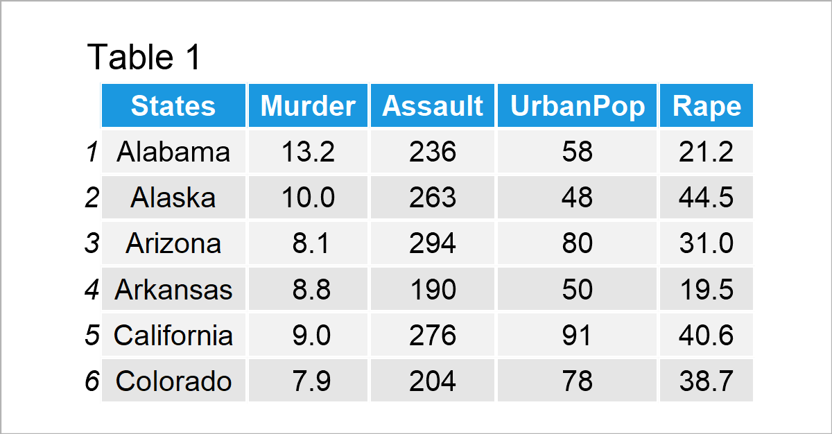
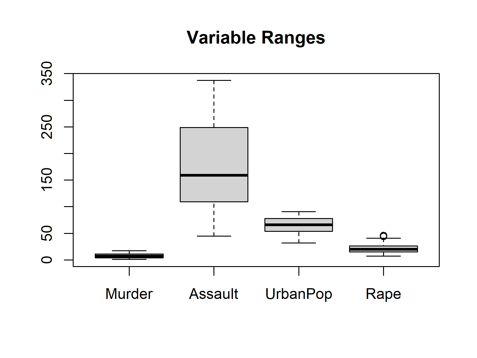
As seen above, the variables have different ranges of values, especially Assault vs. the others. This difference in variation is problematic for getting unbiased results. The variables having larger variations will contribute more to identifying the principal components, even though they are less or equally associated with the component compared to the others.

The next section will show the results obtained using the covariance matrix.

PCA Using Covariance Matrix

Using the covariance between the variables, the loadings showing the association between variables and components are calculated. If you wonder how to compute them in R and Python, see the tutorials: PCA in R and PCA in Python.

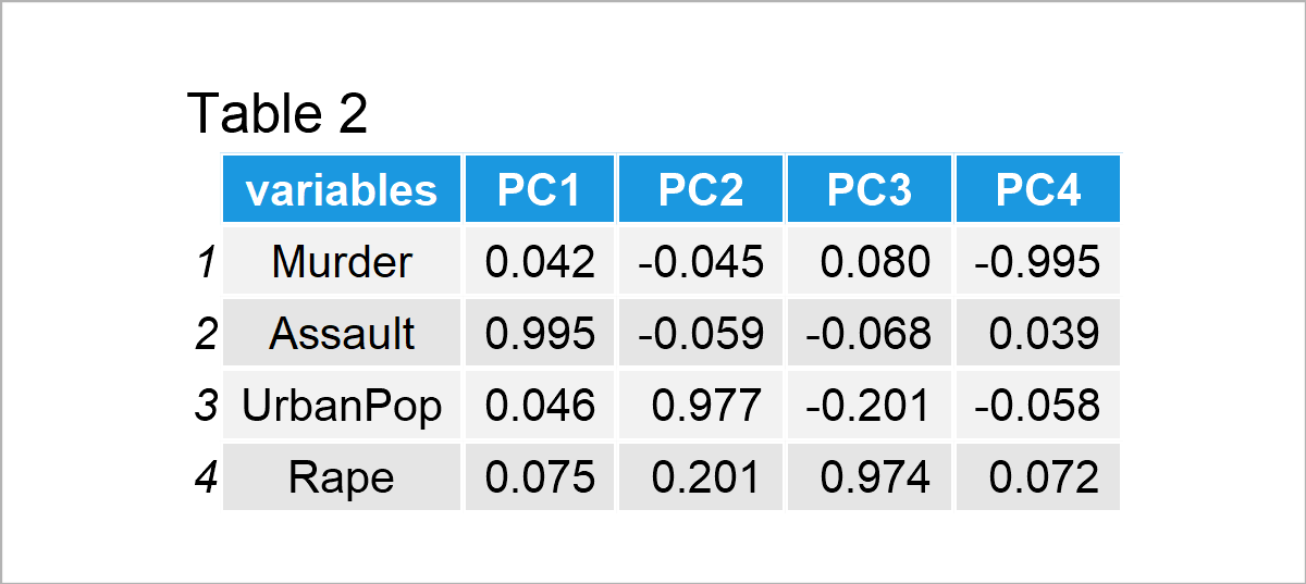
Table 2 shows that each component is strongly associated with only one variable; hence, each component mainly represents a single variable. Assuming 2 principal components will be kept in the analysis, see Optimal Number of Components for details. We can plot our biplot to interpret the results! To learn more about plotting a biplot in R and Python, see the Biplot in R and Biplot in Python tutorials.

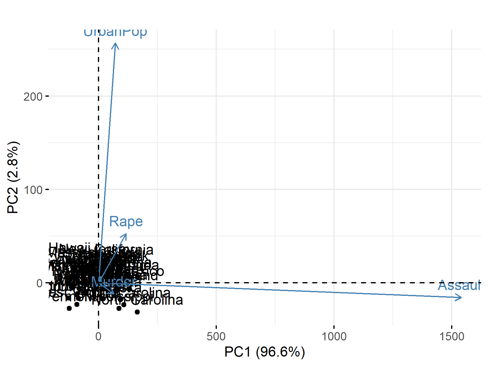
The figure shows that the first and second components explain the variance at 96% and 2.8%. Furthermore, the first principal component splits the states in two as the states with higher assault rates and lower assault rates, whereas the second principal component splits them into the states with the higher and lower urban population.

However, one can argue that the second principal component is not worth considering as it only accounts for about 3% of the variance. Hence we can say that the variation in the dataset can be explained by PC1 only or simply by the assault rates as keeping the PCA out of context. If you would like to know more about how to interpret biplots, you can check our Biplot Explained tutorial.

Let’s see now if this interpretation reflects reality or could be biased due to the unscaled data!

PCA Using Correlation Matrix

Using the correlation matrix is equivalent to using the covariance matrix of the standardized data, which refers to the data with scaled variables having the means of 0s and standard deviations of 1s. Based on the correlation matrix, the following loadings are calculated.

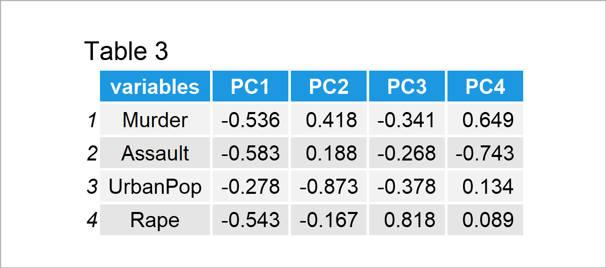
Table 3 shows that each component is strongly associated with multiple variables, which means that more than one variable contribute to identifying each component in contrast to the previous case. Assuming 2 principal components will be kept in the analysis, the following biplot is plotted.

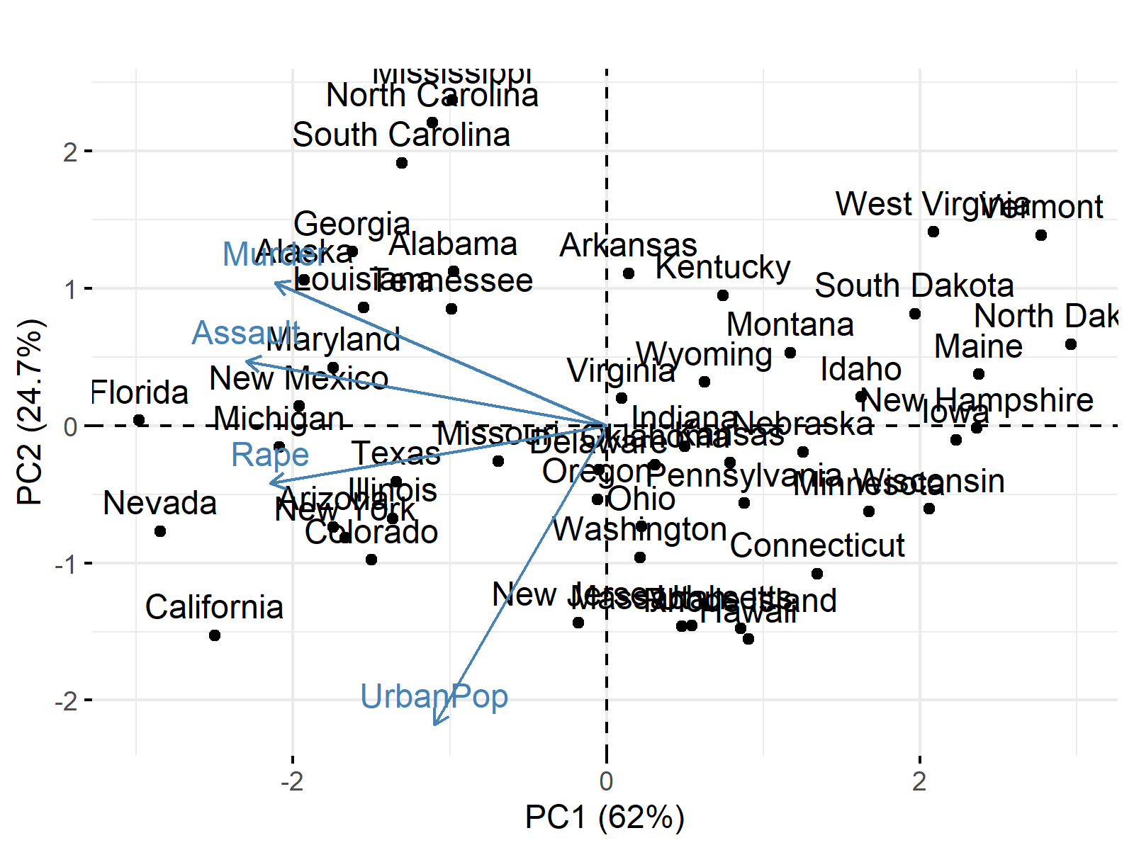
The figure shows that the first and second components account for a considerable amount of variance, and each represents different features that categorize the states.

PC1 divides the states into the states with higher murder, assault, and rape rates and urban populations and those with the opposite. PC2 divides the states into the states with higher rape rates and urban populations, yet lower murder and assault rates, and the states with higher murder and assault rates, yet lower rape rates and urban populations.

As seen, pretty different conclusions can be made based on the choice of input matrix; therefore, we suggest standardizing the data before PCA in case of unequal variation in the dataset.

Video, Further Resources & Summary

Do you need more explanations on the theoretical background of a PCA? Then you should have a look at the following YouTube video of the Statistics Globe YouTube channel.

You can also check some other tutorials on Statistics Globe:

• What is a Principal Component Analysis?
• Choose Optimal Number of Components for PCA
• Principal Component Analysis (PCA) in R
• Principal Component Analysis in Python
• Advantages & Disadvantages of Principal Component Analysis (PCA)
• Biplot for PCA Explained
• Biplot of PCA in R
• Draw Biplot of PCA in Python

This post has shown the differences between performing a PCA with a correlation matrix and a covariance matrix. In case you have further questions, you may leave a comment below.