Introduction to pandas Library in Python (Tutorial & Examples)
In this post, I’ll demonstrate how to handle DataFrames using the pandas library in Python.
I’ll show you detailed instructions and examples on how to manipulate, analyze, visualize, and share your data.
I’ll begin with the basics and move on to more advanced concepts later on. So if you are new to Python or the pandas library, this is the right place to start learning!
The table of contents looks like this:
With that, let’s dig in.
What is pandas?
pandas is an add-on software library created by Wes McKinney for the Python programming language.
The main scope of the pandas library is the manipulation of data sets, i.e. to edit, change, and replace particular elements of a DataFrame class object.
However, pandas provides a broad range of functions and can also be used for other tasks such as the calculation of descriptive statistics and the visualization of the columns and rows in a data set.
Similar to other Python libraries, packages, and modules, pandas is open source, i.e. freely available for usage, modification, and redistribution.
You may find more information on the pandas library on its official website.
In the following part of this tutorial, I’ll demonstrate some example applications of the pandas library in practice.
For this, we first need to load pandas:
import pandas as pd # Import pandas library to Python
After running the previous line of code, we are set up and can start using pandas.
So without further ado, let’s dive into the Python code!
pandas DataFrame Manipulation in Python
This section shows some of the main features of the pandas library. I’ll explain how to add, remove, replace, and merge different data sources.
Let’s do this!
Create Empty pandas DataFrame
As a very first step, we have to create some example data.
For this task, the pandas library provides the DataFrame constructor.
We can create an empty pandas DataFrame using the Python code below:
data1 = pd.DataFrame()                             # Create empty DataFrame
print(data1)                                       # Print empty DataFrame
# Empty DataFrame
# Columns: []
# Index: []
Looks good! Usually, we want to work with some actual values though, so let’s move on!
Create pandas DataFrame with Values
The following code shows how to create a new pandas DataFrame containing several rows and columns:
data2 = pd.DataFrame({'x1':[5, 1, 2, 7, 5, 4],     # Create pandas DataFrame with values
                      'x2':range(1, 7),
                      'x3':['a', 'b', 'a', 'c', 'b', 'c']})
print(data2)                                       # Print pandas DataFrame
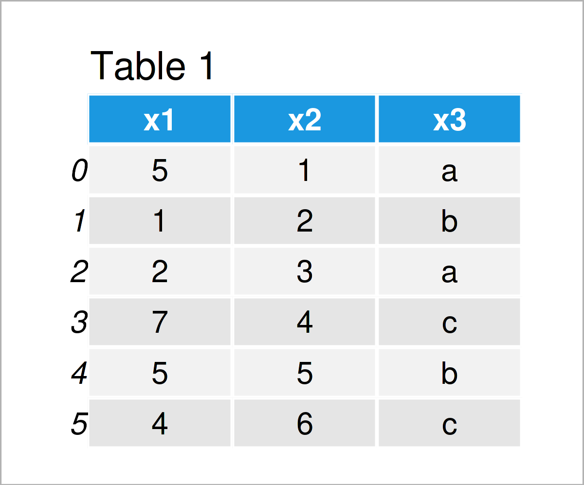
Table 1 illustrates the structure of the previously created pandas DataFrame. As you can see, our example data contains six rows as well as the three columns x1, x2, and x3.
Please keep the structure of this DataFrame in mind, we will use it as a basis for several of the subsequent examples.
Remove Column from pandas DataFrame
The following Python programming syntax demonstrates how to delete a specific variable from a pandas DataFrame.
To accomplish this, we can apply the drop method as shown below:
data3 = data2.drop('x2', axis = 1)                 # Apply drop() function
print(data3)                                       # Print new pandas DataFrame

As shown in Table 2, the previous Python syntax has created a new pandas DataFrame containing only the columns x1 and x3. The column x2 has been excluded.
Select Particular Columns of pandas DataFrame
We can also create DataFrame subsets the other way around as in the previous example. The following Python syntax shows how to select particular columns of a data set.
For this task, we can use double square brackets:
data4 = data2[['x1', 'x2']]                        # Subset columns of pandas DataFrame
print(data4)                                       # Print new pandas DataFrame
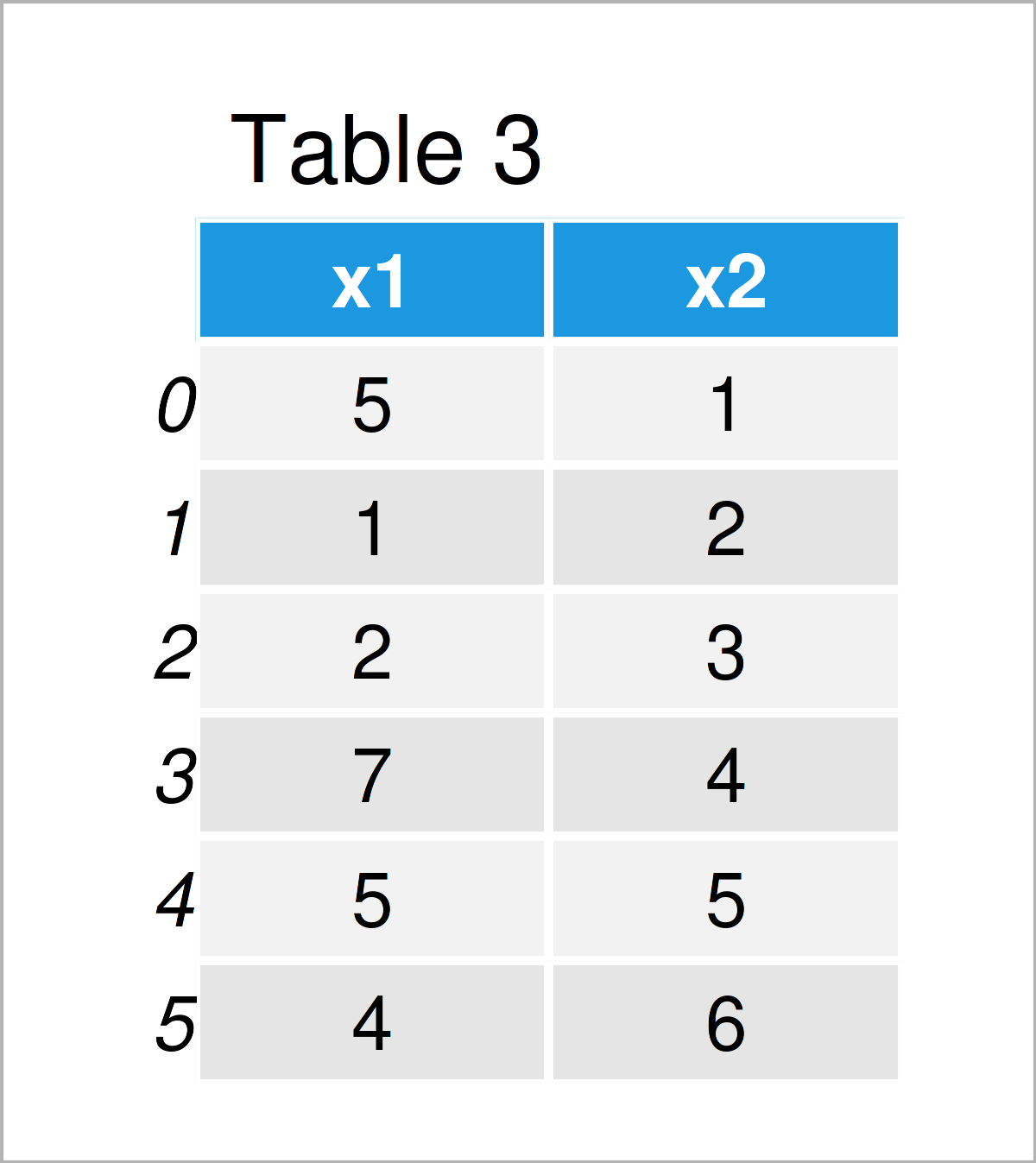
In Table 3 you can see that we have created another pandas DataFrame using the previous Python programming code. This time, we have specified to keep only the variables x1 and x2.
Add Column to pandas DataFrame
This example illustrates how to append a new column to an already existing pandas DataFrame.
For this example, we first need to create a list object that we can add as a new column later:
new_col = [9, 99, 999, 99, 9, 999]                 # Create list
print(new_col)                                     # Print list
# [9, 99, 999, 99, 9, 999]
Next, we can apply the assign function to union our pandas DataFrame called data4 (that we have created in the previous example) with our list:
data5 = data4.assign(new_col = new_col)            # Add list as new column to DataFrame
print(data5)                                       # Print new pandas DataFrame

Table 4 shows the output of the previous Python programming code – Another pandas DataFrame where we have added a list as a new column.
Change Data Type of pandas DataFrame Column
It is important to know that pandas DataFrame columns (as well as other data objects) can have different data types.
This example explains how to modify the data type of a certain pandas DataFrame column.
Let’s first create a copy of our DataFrame data5:
data6 = data5.copy() # Create copy of pandas DataFrame
Next, let’s check the data classes of all the columns in our DataFrame. We can do that using the dtypes attribute:
print(data6.dtypes)                                # Print types of all columns
# x1         int64
# x2         int64
# new_col    int64
# dtype: object
At this point, all our columns are integers (represented by int64).
Let’s assume that we want to convert the column new_col from the integer data type to a character string. Then, we can apply the astype function as shown below:
data6['new_col'] = data6['new_col'].astype(str)    # Convert column to string
print(data6)                                       # Print new pandas DataFrame
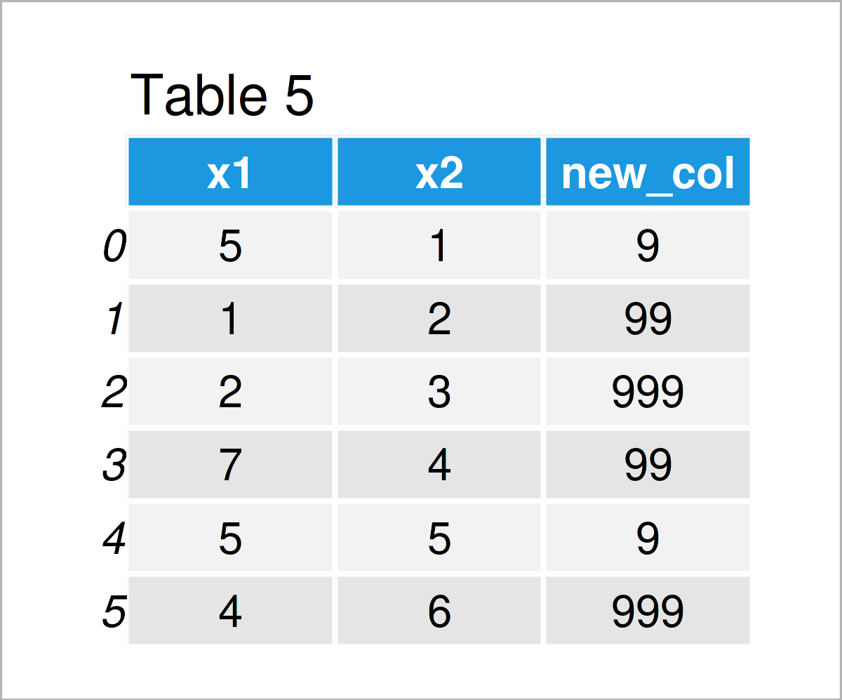
In Table 5 you can see that our new pandas DataFrame looks exactly the same as the input DataFrame, even though we have changed the data type.
However, you can see the difference by printing the data types of our DataFrame columns once again to the console:
print(data6.dtypes)                                # Print types of all columns
# x1          int64
# x2          int64
# new_col    object
# dtype: object
Compare this output with the previous output above. As you can see, the data type column new_col has been changed to the string class (represented by “object”).
Merge Two pandas DataFrames
So far, we have dealt with only one pandas DataFrame. However, sometimes you might face two or more data sets.
This example illustrates how to merge multiple data sets into a single pandas DataFrames.
As preparation for this example, we first have to create two new pandas DataFrames:
data7 = pd.DataFrame({'ID':range(1001, 1007),      # Create first pandas DataFrame with ID
                      'x1':[5, 1, 2, 7, 5, 4],
                      'x2':range(1, 7),
                      'x3':['a', 'b', 'a', 'c', 'b', 'c']})
print(data7)                                       # Print pandas DataFrame
data8 = pd.DataFrame({'ID':range(1004, 1011),      # Create second pandas DataFrame with ID
                      'y1':range(10, 3, - 1),
                      'y2':['x', 'y', 'y', 'x', 'x', 'y', 'x']})
print(data8)                                       # Print pandas DataFrame
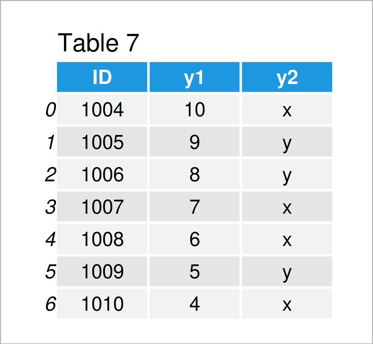
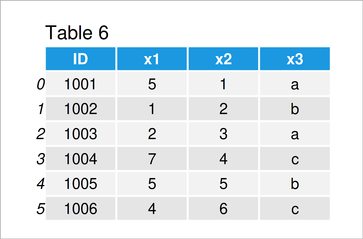
The output of the previous Python programming code is shown in Tables 7 and 8. We have constructed two new pandas DataFrames that both contain an ID column.
In the next step, we can use this ID column and the merge function to combine our two pandas DataFrames horizontally:
data9 = pd.merge(data7,                            # Inner join
                 data8,
                 on = 'ID')
print(data9)                                       # Print merged pandas DataFrame

In Table 8 it is shown that we have created a merged pandas DataFrame with the previous Python programming syntax.
You might already have noticed that the merged DataFrame contains much fewer rows than our two input data sets.
The reason for this is that the two input DataFrames contain different IDs. In the previous Python code, we have used a so-called inner join, which keeps only those IDs that are contained in both input data sets.
Alternatively, we might apply an outer join by specifying the how argument to be equal to “outer”:
data10 = pd.merge(data7,                           # Outer join
                  data8,
                  on = 'ID',
                  how = 'outer')
print(data10)                                      # Print merged pandas DataFrame
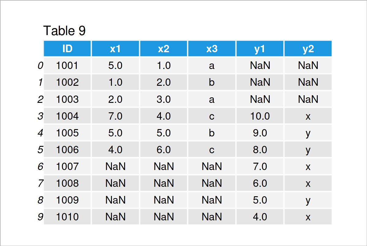
By running the previous Python syntax, we have constructed Table 9, i.e. a merged pandas DataFrame with as many rows as possible.
Those IDs that were only contained in one of the input DataFrame were set to NaN for the columns of the other input DataFrame.
To select the right type of join is crucial for the later data analysis. If you want to learn more about different joins, you may have a look here.
Rename Columns of pandas DataFrame
We can also adjust the names of the columns in a pandas DataFrame in Python.
For this task, we can use the columns attribute as shown below:
data11 = data9.copy()                              # Create copy of pandas DataFrame
data11.columns = ['ID', 'col1', 'col2', 'col3', 'col4', 'col5'] # Rename columns of DataFrame
print(data11)                                      # Print updated pandas DataFrame

In Table 10 you can see that we have created another pandas DataFrame with different column names by executing the previous Python syntax.
Remove Row from pandas DataFrame
Until this point of the tutorial, we have mainly focused on the columns of a pandas DataFrame. However, the pandas library also provides many tools for the manipulation of DataFrame rows.
This section demonstrates how to delete certain rows of a pandas DataFrame based on a logical condition.
To achieve this, we can use square brackets and the != operator as shown in the following Python code:
data12 = data2.copy()                              # Create copy of pandas DataFrame
data12 = data12[data12.x1 != 5]                    # Drop by logical condition
print(data12)                                      # Print updated pandas DataFrame
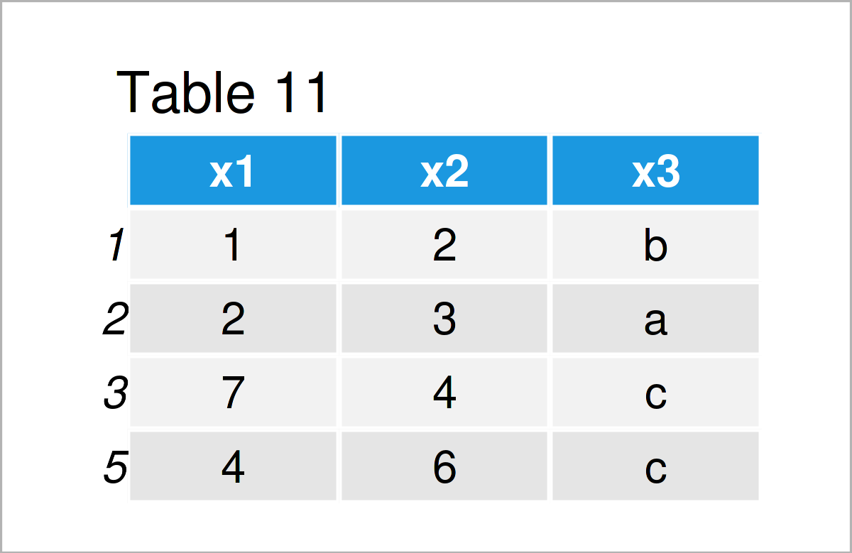
As shown in Table 11, the previous Python programming code has created an updated version of our data set where all rows with the value 5 in the column x1 have been dropped.
Add Row to pandas DataFrame
We can also do the opposite! This example explains how to append a new row at a certain index position to a pandas DataFrame.
Let’s first create a list object that we can add as a new row later:
new_row = [10, 20, 30]                             # Create list
print(new_row)                                     # Print list
# [10, 20, 30]
Next, we can add this list as a new row at the bottom of our data set:
data13 = data12.copy()                             # Create copy of pandas DataFrame
data13.loc[6] = new_row                            # Add list as new row to pandas DataFrame
print(data13)                                      # Print updated pandas DataFrame
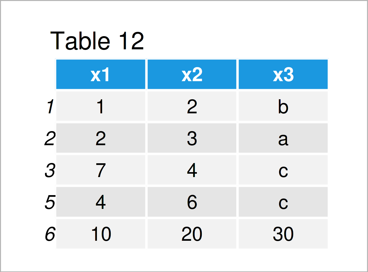
After running the previous Python programming syntax the pandas DataFrame with an additional row at the bottom shown in Table 12 has been created.
Concatenate Two pandas DataFrames
It is also possible to stack several pandas DataFrames on top of each other.
To do this, we can apply the append function. Note that we are also specifying the ignore_index argument to be equal to True, because in this example we want to reset the indices of our updated data set.
data14 = data2.append(data13,                      # Append two pandas DataFrames
                      ignore_index = True)
print(data14)                                      # Print combined pandas DataFrame
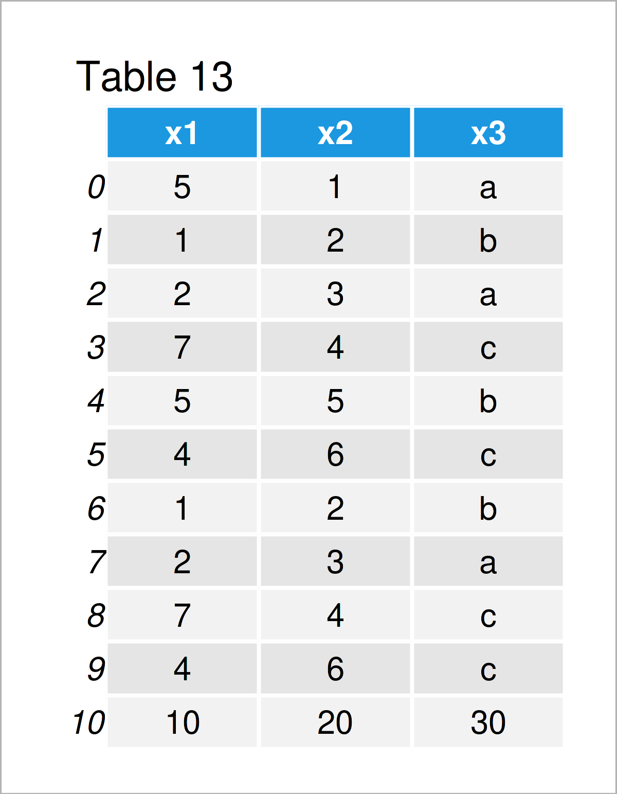
After executing the previous Python programming code the vertically combined DataFrame shown in Table 13 has been created.
Sort Rows of pandas DataFrame
The rows of an already existing pandas DataFrame can also be ordered based on the values in a certain column of this DataFrame.
data15 = data14.copy()                             # Create copy of pandas DataFrame
data15 = data15.sort_values('x1')                  # Order Rows of pandas DataFrame
print(data15)                                      # Print updated pandas DataFrame

The output of the previous Python code is shown in Table 14: An updated pandas DataFrame where the rows have been sorted based on the values in the column x1.
Change Row Indices of pandas DataFrame
You might already have wondered what the values on the left side of the rows in our pandas DataFrames mean. These values are called the index of a pandas DataFrame.
This example explains how to reset the index values of a pandas DataFrame.
Remember the data set shown in Table 14 that we have created in the previous example. As you can see, the indices of this data set are not formatted by a certain range.
If we want to reset the index values of this pandas DataFrame, we can use the reset_index method as shown below:
data16 = data15.reset_index(drop = True)           # Reset index of pandas DataFrame
print(data16)                                      # Print updated pandas DataFrame

In Table 15 you can see that we have created a new pandas DataFrame where the index values are ranging from 0 to the number of rows in our data set.
Iterate Through Rows of pandas DataFrame
A commonly used feature in Python a for loops.
We can use such loops to iterate over the rows in a pandas DataFrame.
The Python code below demonstrates how to print an output for each DataFrame row by iterating through the lines of our pandas DataFrame data2.
Consider the Python syntax and its output below:
for i, row in data2.iterrows():                    # Iterate over rows of pandas DataFrame
    print(row['x1'], '* 3 =', row['x1'] * 3)
# 5 * 3 = 15
# 1 * 3 = 3
# 2 * 3 = 6
# 7 * 3 = 21
# 5 * 3 = 15
# 4 * 3 = 12
As you can see, we have printed some output for each line of our data set.
Summary Statistics of pandas DataFrame
The previous section has explained how to prepare and edit the shape of your data depending on your specific needs. Once this step is done, the typically next step is the analysis of your data by applying different statistical methods.
This section gives a brief overview on how to calculate some of the most important summary statistics for your data.
Let’s jump right in!
Calculate Descriptive Statistics for pandas DataFrame
In this part of the tutorial, I want to show you the calculation of some basic descriptive metrics for the entire columns of a pandas DataFrame.
Let’s start with the mean!
We can compute the mean for all the numeric columns in a pandas DataFrame by applying the mean function as demonstrated below:
print(data2.mean())                                # Get mean of all numeric columns
# x1    4.0
# x2    3.5
# dtype: float64
As you can see, the mean of the column x1 is 4.0 and the mean of the column x2 is 3.5. The previous Python syntax has not returned a value for the column x3, since this column contains strings.
We can exchange the mean function by other functions that are designed to compute descriptive statistics.
The following code uses the max function to return the maximum value of each column:
print(data2.max())                                 # Get maximum of all columns
# x1    7
# x2    6
# x3    c
# dtype: object
The maximum value of the column x1 is 7, and the maximum value of the column x2 is 6. In contrast to the mean function, the max function also prints an output for string variables, i.e. the character “c” is the latest letter in the alphabet that occurs in this column.
We may now use other functions to calculate even more summary stats for our data. However, the pandas library fortunately provides the describe function to return an output that consists of multiple descriptive statistics.
Let’s do this:
print(data2.describe())                            # Get multiple descriptive statistics
#             x1        x2
# count  6.00000  6.000000
# mean   4.00000  3.500000
# std    2.19089  1.870829
# min    1.00000  1.000000
# 25%    2.50000  2.250000
# 50%    4.50000  3.500000
# 75%    5.00000  4.750000
# max    7.00000  6.000000
As you can see, the previous code has returned the count, mean, standard deviation, minimum, quantiles, and maximum values for all the numeric columns.
Easy peasy!
Aggregate pandas DataFrame by Group
In the previous section, we have calculated descriptive statistics for entire DataFrame columns. However, quite often it is useful to analyze data by group.
The Python code below shows how to get the mean by group for each numeric column in our data set. Note that we are using the column x3 to divide our data into several groups:
print(data2.groupby('x3').mean())                  # Get mean by group
#      x1   x2
# x3
# a   3.5  2.0
# b   3.0  3.5
# c   5.5  5.0
The previous output shows a matrix containing a mean value for each column and each group.
Similar to the previous code, we can use the describe function to return multiple descriptive statistics for each group in each column of our data:
print(data2.groupby('x3').describe())              # Get mean by group
#       x1                                 ...        x2
#    count mean       std  min   25%  50%  ...       std  min   25%  50%   75%  max
# x3                                       ...
# a    2.0  3.5  2.121320  2.0  2.75  3.5  ...  1.414214  1.0  1.50  2.0  2.50  3.0
# b    2.0  3.0  2.828427  1.0  2.00  3.0  ...  2.121320  2.0  2.75  3.5  4.25  5.0
# c    2.0  5.5  2.121320  4.0  4.75  5.5  ...  1.414214  4.0  4.50  5.0  5.50  6.0
#
# [3 rows x 16 columns]
Our outputs start to become more complex – However, I hope you still get the point of this! 🙂
Draw Plot of pandas DataFrame
Enough of numbers?! No worries, the next section focuses on the creation of graphics based on pandas DataFrames.
Note that the following graphics will be created by the matplotlib library, which is automatically available when using the pandas library.
We can use the plot function to draw various types of different graphs. The type of graph can be specified by the kind argument. In addition, we may specify the specific variables of our DataFrame that we want to draw.
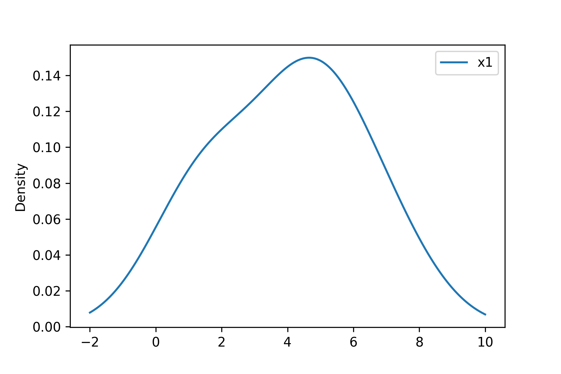
The Python syntax below creates a density plot of the column x1:
data2.plot(kind = 'density', y = 'x1') # Draw density plot
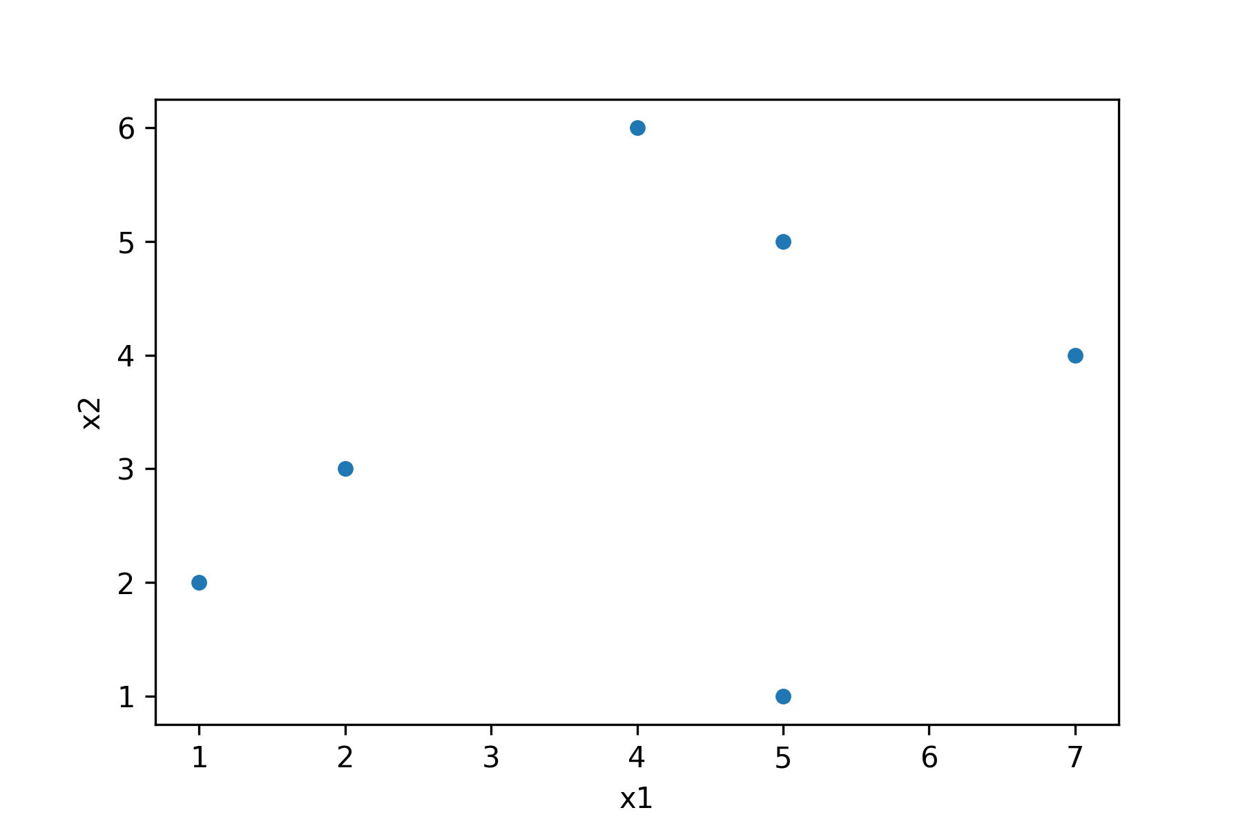
Similar to that, we can create a plot showing two variables. The following Python code visualizes the columns x1 and x2 in a scatterplot:
data2.plot(kind = 'scatter', x = 'x1', y = 'x2') # Draw scatterplot
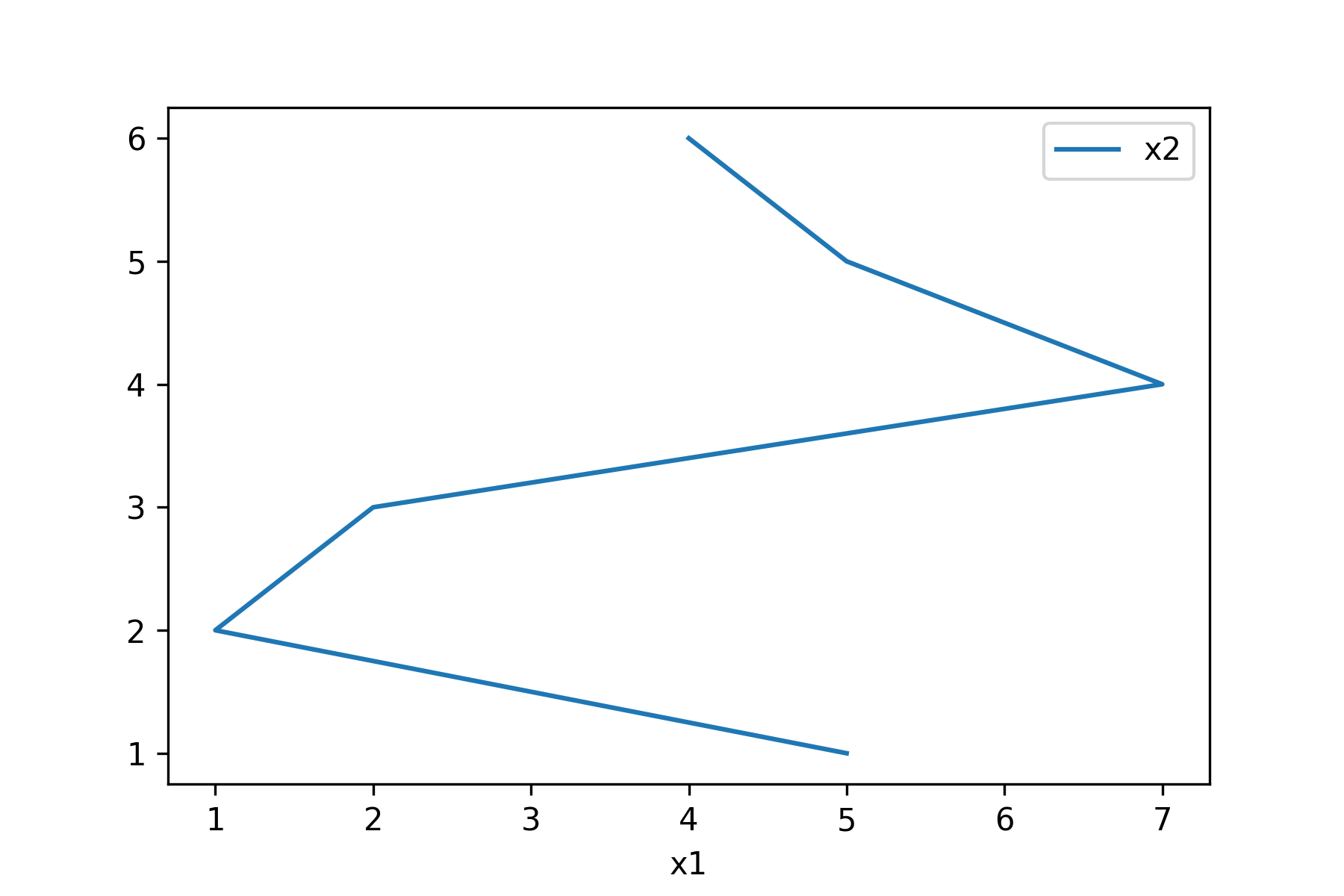
If we specify the kind argument to be equal to “line”, a line plot is drawn:
data2.plot(kind = 'line', x = 'x1', y = 'x2') # Draw line plot
A barchart can be created using the following code:
data2.plot(kind = 'bar', y = 'x1') # Draw barplot
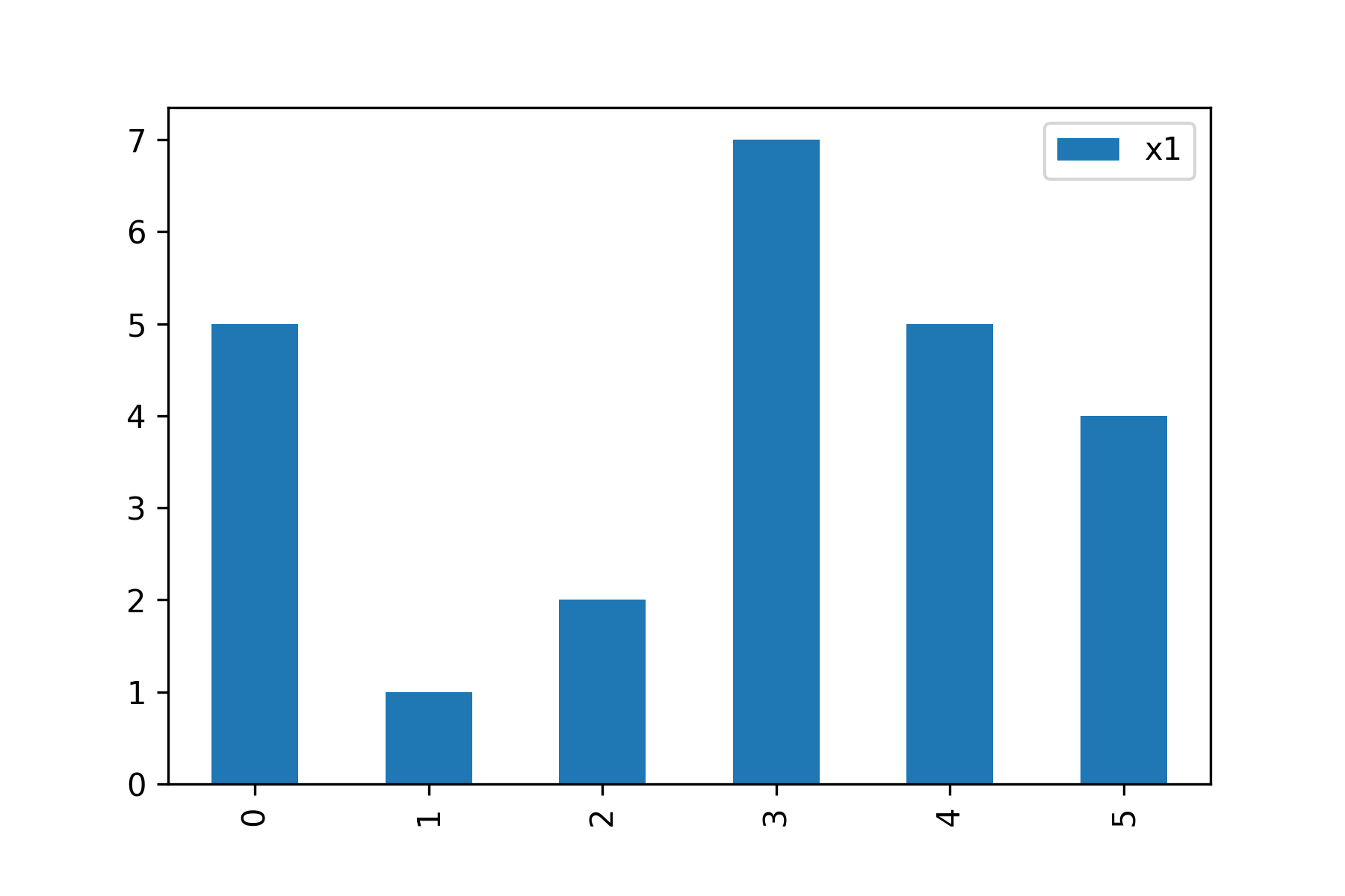
And last, but not least, we can draw multiple boxplots side-by-side using the syntax below:
data2.plot(kind = 'box') # Draw boxplot
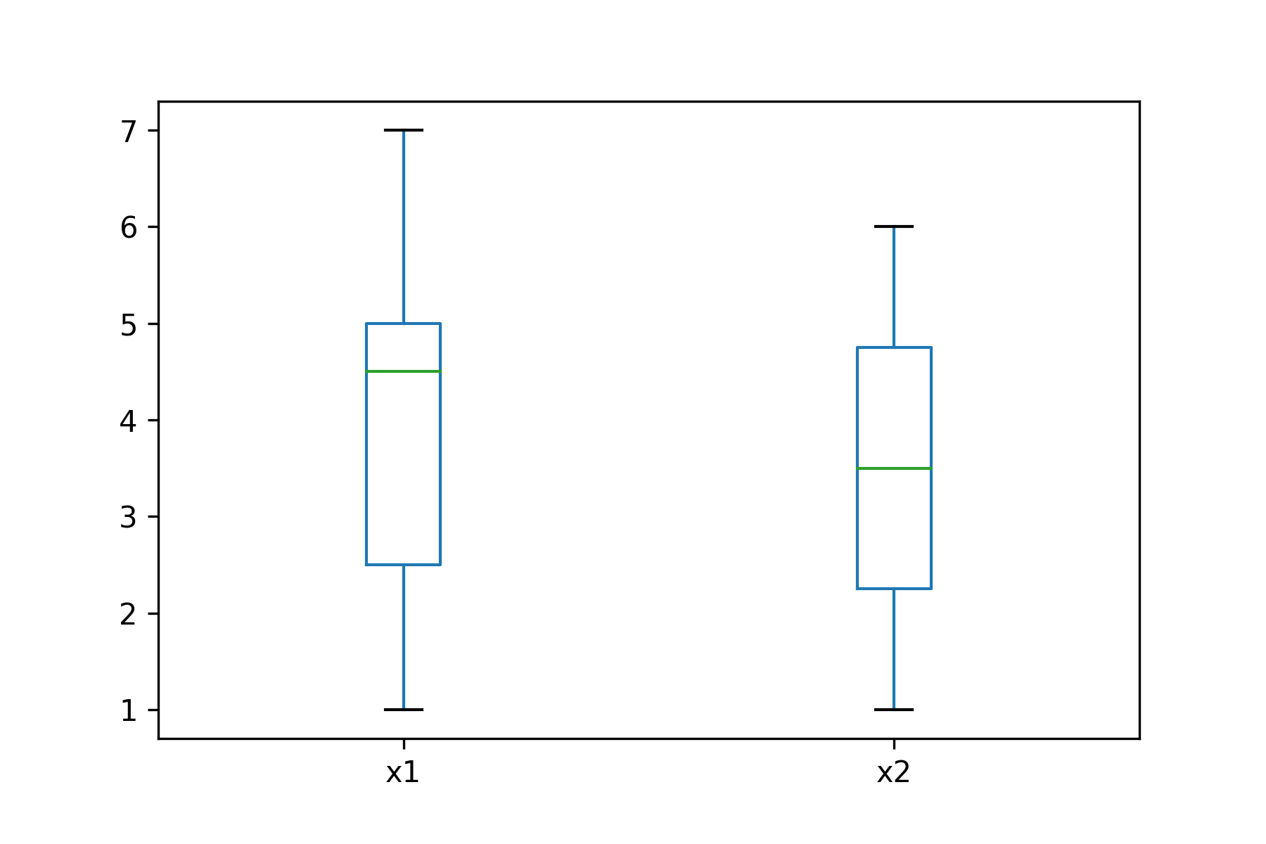
The previous plots are only a tiny selection of various types of graphics that are provided by pandas and the matplotlib libraries. Please have a look here, for a broader overview.
Export / Import pandas DataFrame to / from External File
To wrap up the examples of this pandas introduction tutorial, I want to show you how to store and import pandas DataFrames in / from external files.
This is often the final step when preparing your data for other users, or to have a final output that can be loaded back in in another script in your next Python session.
The following examples show how to write and read pandas DataFrames to / from CSV files. However, other file formats could also be used.
Write pandas DataFrame to CSV File
This example shows how to save a pandas DataFrame as a CSV file on your computer.
To accomplish this, we first have to import the os module:
import os # Import os module in Python
Furthermore, we have to specify the working directory to which we want to export our data. In this case, I have created a working directory called “my directory” on the desktop of my computer.
os.chdir('C:/Users/Joach/Desktop/my directory') # Set working directory
In the next step, we can apply the to_csv function to write our pandas DataFrame to a CSV file in our working directory. Note that we are also specifying the file name that we want to use; and we are setting the index argument to be equal to False, because I prefer not to export the indices of our data as a separate column.
data2.to_csv('data2.csv',                          # Export pandas DataFrame to CSV file
             index = False)
After executing the previous syntax, a new CSV file appears in my working directory. This file can be shared or used by myself, the next time I want to work with my data.
Read pandas DataFrame from CSV File
Let’s assume that some time has passed by, and we want to load our CSV file back to a new Python session as a pandas DataFrame.
Then, we can use the read_csv function as shown below. Note that we would have to set the working directory to the folder path where our data is stored once again (see the previous section), in case we have not done so yet.
Have a look at the Python code and its output below:
data17 = pd.read_csv('data2.csv')                  # Import pandas DataFrame from CSV file
print(data17)
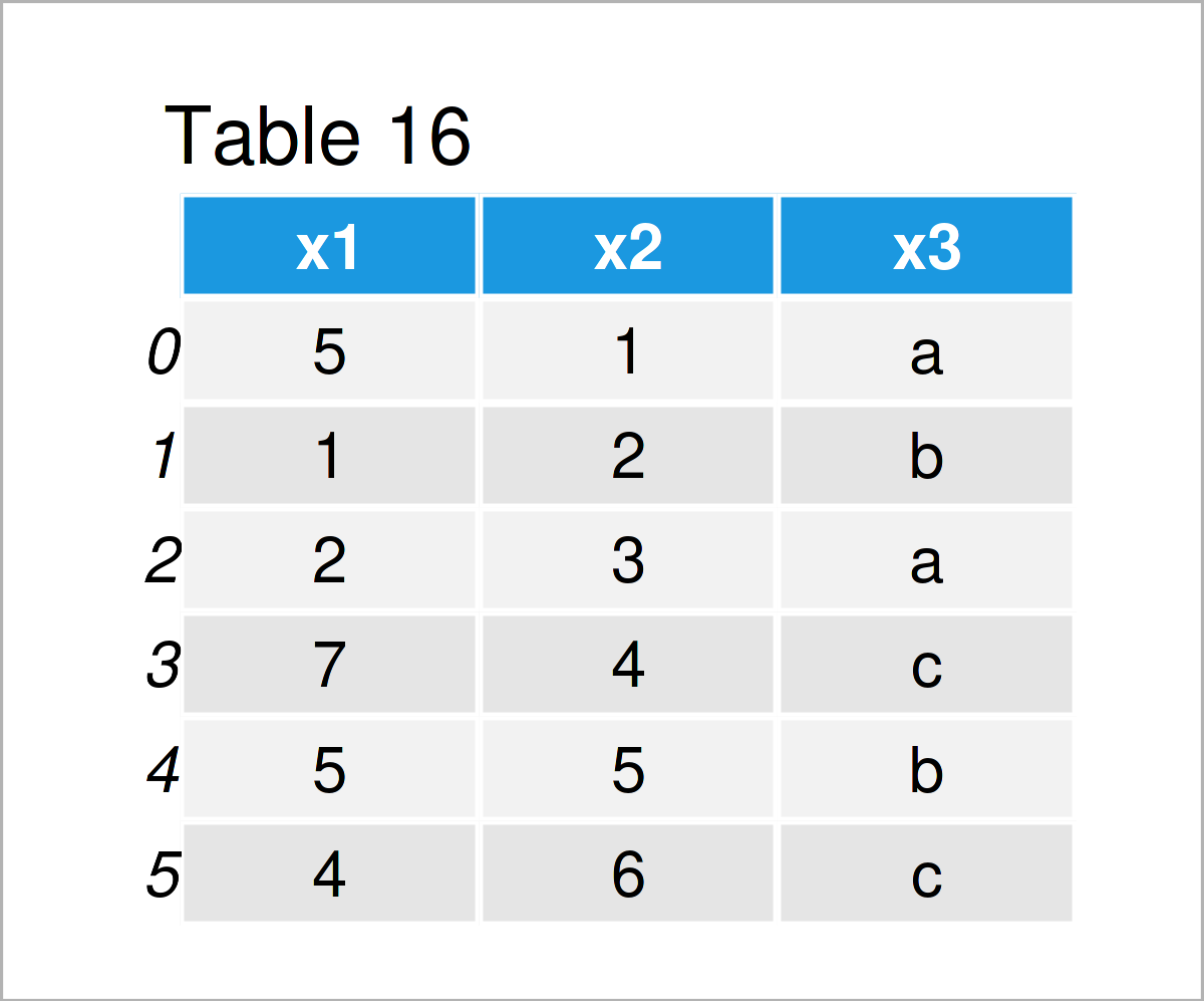
The output of the previous syntax is shown in Table 16 – We have imported our CSV file, and we have stored it in a new pandas DataFrame object called data17.
Now, we can start working on this data set again – great!
Video & Further Resources
Would you like to learn more about the wrangling of DataFrames using the pandas library? Then you might have a look at the following video that I have published on my YouTube channel. I’m explaining the topics of this post in the video.
In addition, you could have a look at the other posts on the pandas library on this website. They show the concepts of the present introduction in some more detail.
Please find a complete list of all tutorials for beginners and advanced Python users below:
To summarize: This free introduction course has explained the basics on how to deal with DataFrames using the pandas library in Python programming. If you have any further questions, don’t hesitate to let me know in the comments section.
Subscribe to the Statistics Globe Newsletter
Get regular updates on the latest tutorials, offers & news at Statistics Globe.
I hate spam & you may opt out anytime: Privacy Policy.
Thank you!
Welcome to the Statistics Globe newsletter. From now on, I’ll send you regular emails about statistics, data science, AI, and programming with R and Python.
I’m Joachim Schork. On this website, I provide statistics tutorials as well as code in Python and R programming.
Statistics Globe Newsletter
Get regular updates on the latest tutorials, offers & news at Statistics Globe. I hate spam & you may opt out anytime: Privacy Policy.
Thank you!
Please check your email inbox and click the confirmation link to complete your subscription. If you don’t see the email within a few minutes, please also check your spam/junk folder.


