Data Cleaning in R (9 Examples)

In this R tutorial you’ll learn how to perform different data cleaning (also called data cleansing) techniques.

The tutorial will contain nine reproducible examples. To be more precise, the content is structured as follows:

Let’s do this…

Creation of Example Data

We use the following data as a basis for this R programming tutorial:

data <- data.frame(x1 = c(1:4, 99999, 1, NA, 1, 1, NA),   # Create example data frame
                   x1 = c(1:5, 1, "NA", 1, 1, "NA"),
                   x1 = c(letters[c(1:3)], "x  x",  "x", "   y    y y", "x", "a", "a", NA),
                   x4 = "",
                   x5 = NA)
data                                                      # Print example data frame

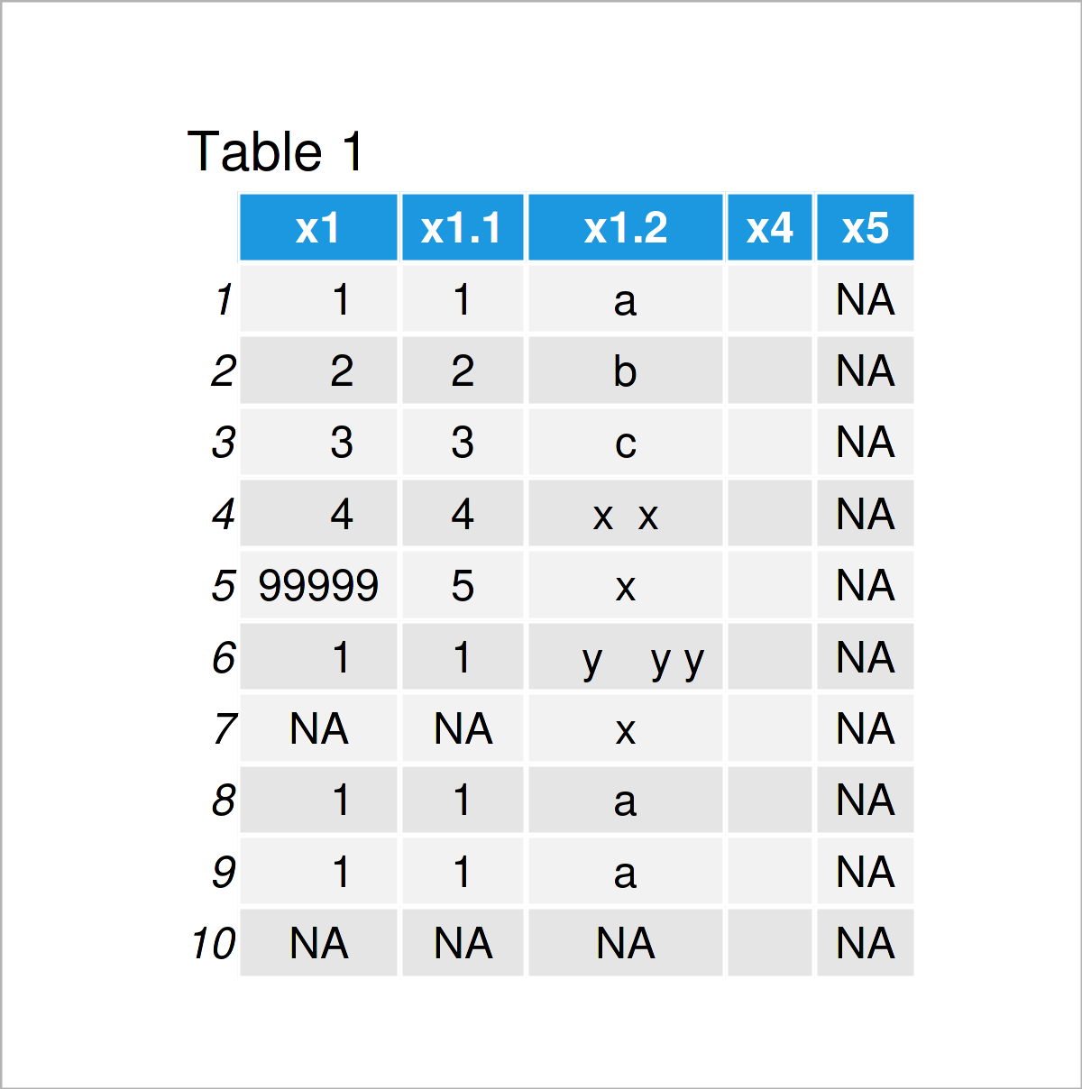
Have a look at the previous table. It visualizes that our exemplifying data is constituted of ten rows and five variables.

As you might already have noticed, some parts of this data set are not formatted properly. In the following examples, I’ll show some tricks on how to edit and improve the structure of this data set.

Let’s dive right into the examples!

Example 1: Modify Column Names

Example 1 explains how to clean the column names of a data frame.

Let’s first have a closer look at the names of our data frame columns:

colnames(data)                                            # Print column names
# [1] "x1"   "x1.1" "x1.2" "x4"   "x5"

Let’s assume that we want to change these column names to a consecutive range with the prefix “col”. Then, we can apply the colnames, paste0, and ncol functions as shown below:

colnames(data) <- paste0("col", 1:ncol(data))             # Modify all column names
data                                                      # Print updated data frame

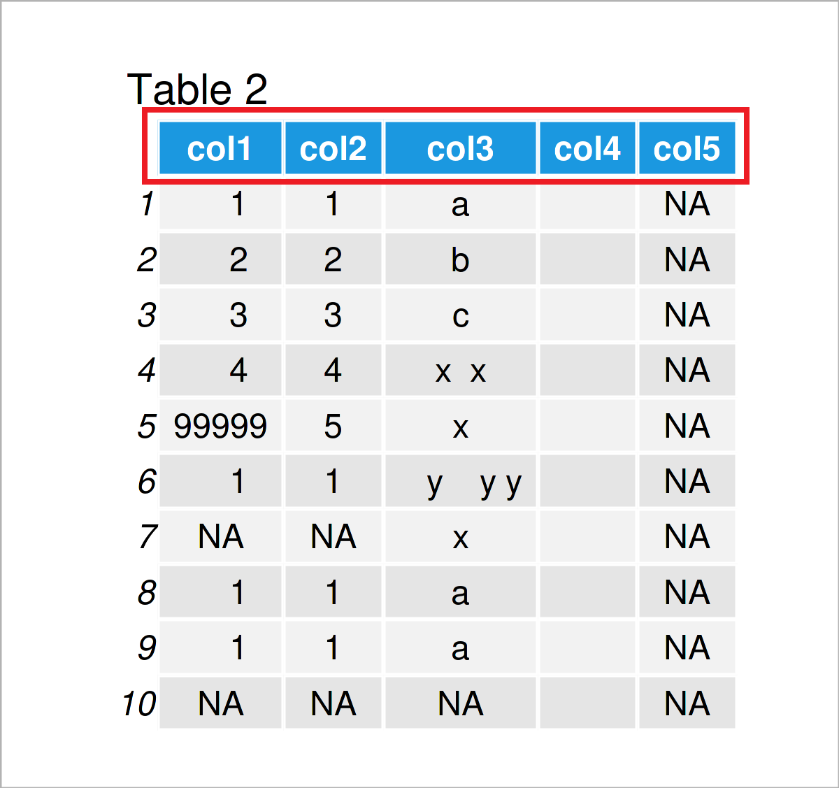
As shown in Table 2, the previous syntax has created an updated version of our data frame where the column names have been changed.

Example 2: Format Missing Values

A typical problem for each data preparation and cleaning task are missing values.

In the R programming language, missing values are usually represented by NA. For that reason, it is useful to convert all missing values to this NA format.

In our specific example data frame, we have the problem that some missing values are represented by blank character strings.

We can print all those blanks to the RStudio console as shown below:

data[data == ""]                                          # Print blank data cells
#  [1] NA NA NA "" "" "" "" "" "" "" "" "" "" NA NA NA NA NA NA NA NA NA NA

If we want to assign NA values to those blank cells, we can use the following syntax:

data[data == ""] <- NA                                    # Replace blanks by NA

Another typical problem with missing values – that also occurs in our data set – is that NA values are formatted as the character string “NA”.

Let’s have a closer look at the column col2:

data$col2                                                 # Print column
#  [1] "1"  "2"  "3"  "4"  "5"  "1"  "NA" "1"  "1"  "NA"

As you can see in the previous output, the NA values in this column are shown between quotes (i.e. “NA”). This indicates that those NA values are formatted as characters instead of real NA values.

We can change that using the following R code:

data$col2[data$col2 == "NA"] <- NA                        # Replace character "NA"

Let’s have another look at our updated data frame:

data                                                      # Print updated data frame

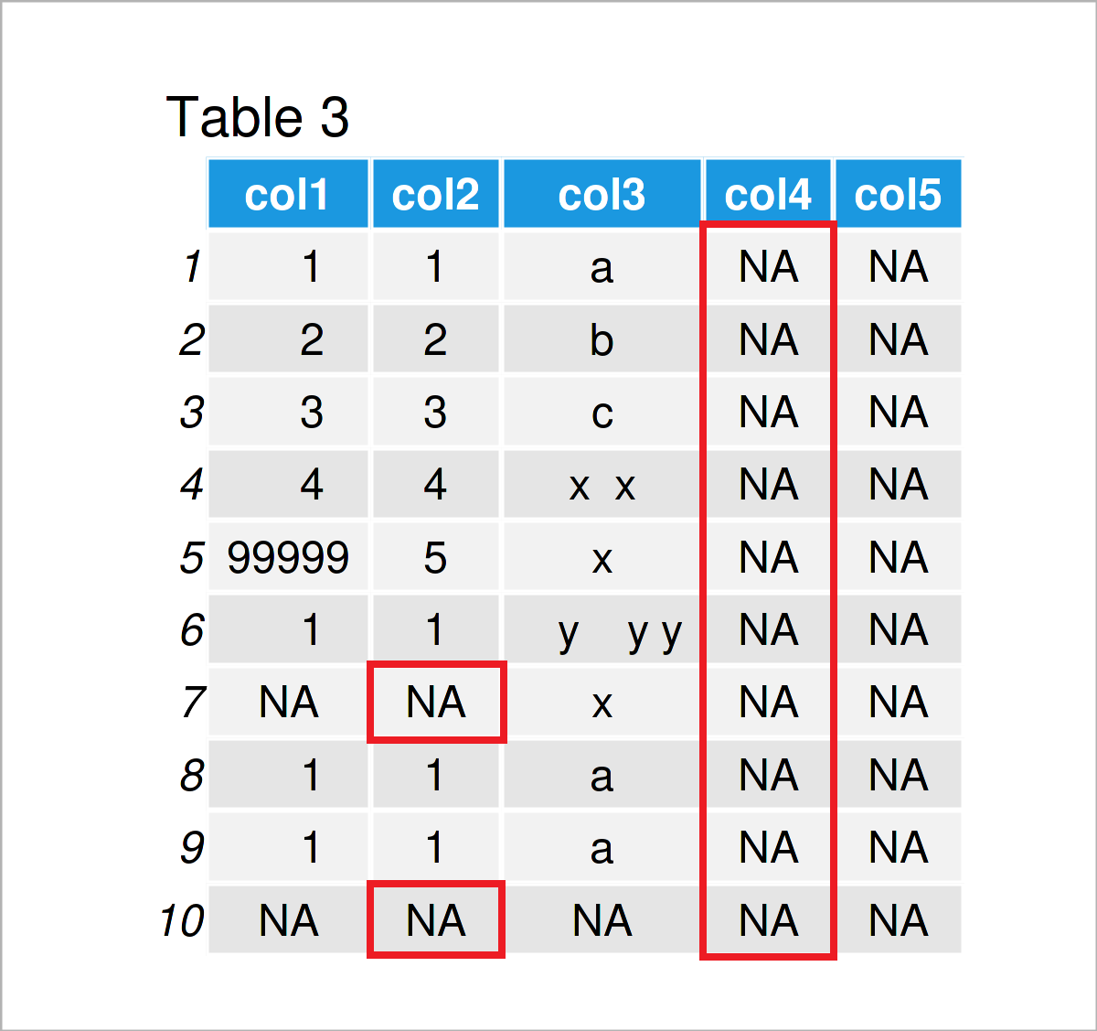
In Table 3 it is shown that we have converted all empty characters “” and all character “NA” to true missing values.

Example 3: Remove Empty Rows & Columns

Example 3 demonstrates how to identify and delete rows and columns that contain only missing values.

On a side note: Example 2 was also important for this step, since the false formatted NA values would not have been recognized by the following R code.

The syntax below demonstrates how to use the rowSums, is.na, and ncol functions to remove only-NA rows:

data <- data[rowSums(is.na(data)) != ncol(data), ]        # Drop empty rows
data                                                      # Print updated data frame

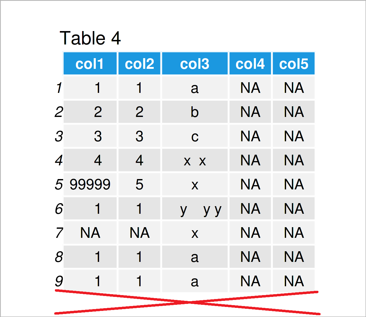
As shown in Table 4, the previous R syntax has kept only rows with non-NA values.

Similar to that, we can also exclude columns that contain only NA values:

data <- data[ , colSums(is.na(data)) != nrow(data)]       # Drop empty columns
data                                                      # Print updated data frame

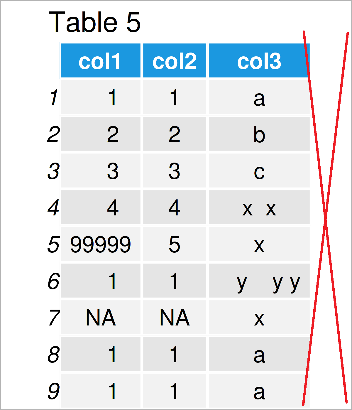
By executing the previous R programming syntax, we have created Table 5, i.e. a data frame without empty columns.

Example 4: Remove Rows with Missing Values

As you can see in the previously shown table, our data still contains some NA values in the 7th row of the data frame.

In this example, I’ll explain how to delete all rows with at least one NA value.

This method is called listwise deletion or complete cases analysis, and it should be done with care! Statistical bias might be introduced to your results, if data is removed without theoretical justification.

However, in case you have decided to remove all rows with one or more NA values, you may use the na.omit function as shown below:

data <- na.omit(data)                                     # Delete rows with missing values 
data                                                      # Print updated data frame

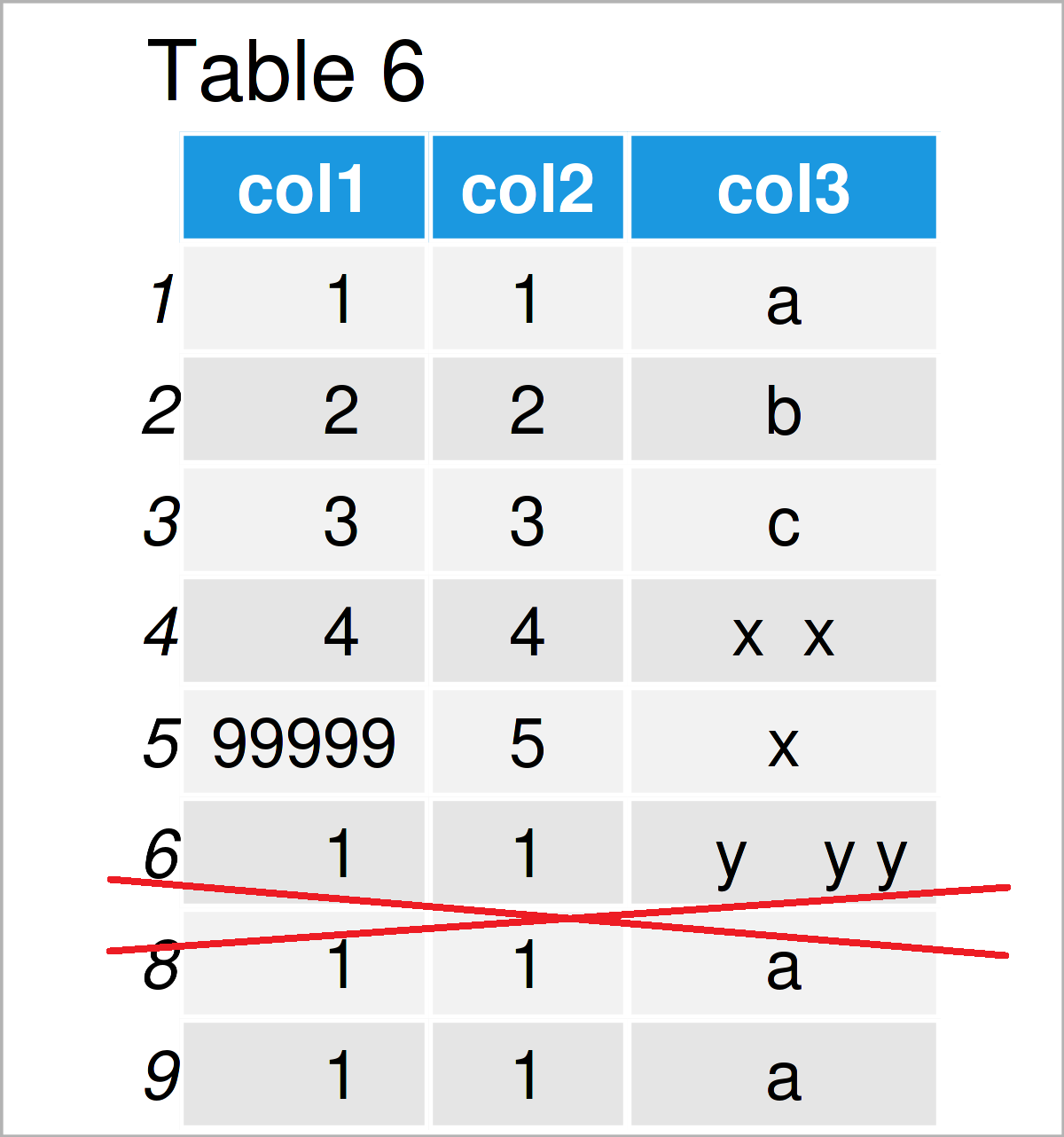
Table 6 shows the output of the previous R programming code: We have removed all rows with missing values.

Example 5: Remove Duplicates

In this example, I’ll demonstrate how to keep only unique rows in a data set.

For this task, we can apply the unique function to our data frame as demonstrated in the following R snippet:

data <- unique(data)                                      # Exclude duplicates
data                                                      # Print updated data frame

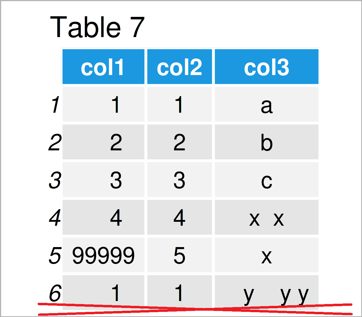
Table 7 visualizes the output of the previous R programming code – We have removed the last two rows from our data since they were duplicates to the first row.

Example 6: Modify Classes of Columns

The class of the columns of a data frame is another critical topic when it comes to data cleaning.

This example explains how to format each column to the most appropriate data type automatically.

Let’s first check the current classes of our data frame columns:

sapply(data, class)                                       # Print classes of all columns
#        col1        col2        col3 
#   "numeric" "character" "character"

The first variable col1 is numeric, and the columns col2 and col3 are characters.

We can now use the type.convert function to change the column classes whenever it is appropriate:

data <- type.convert(data, as.is = TRUE)
data                                                      # Print updated data frame

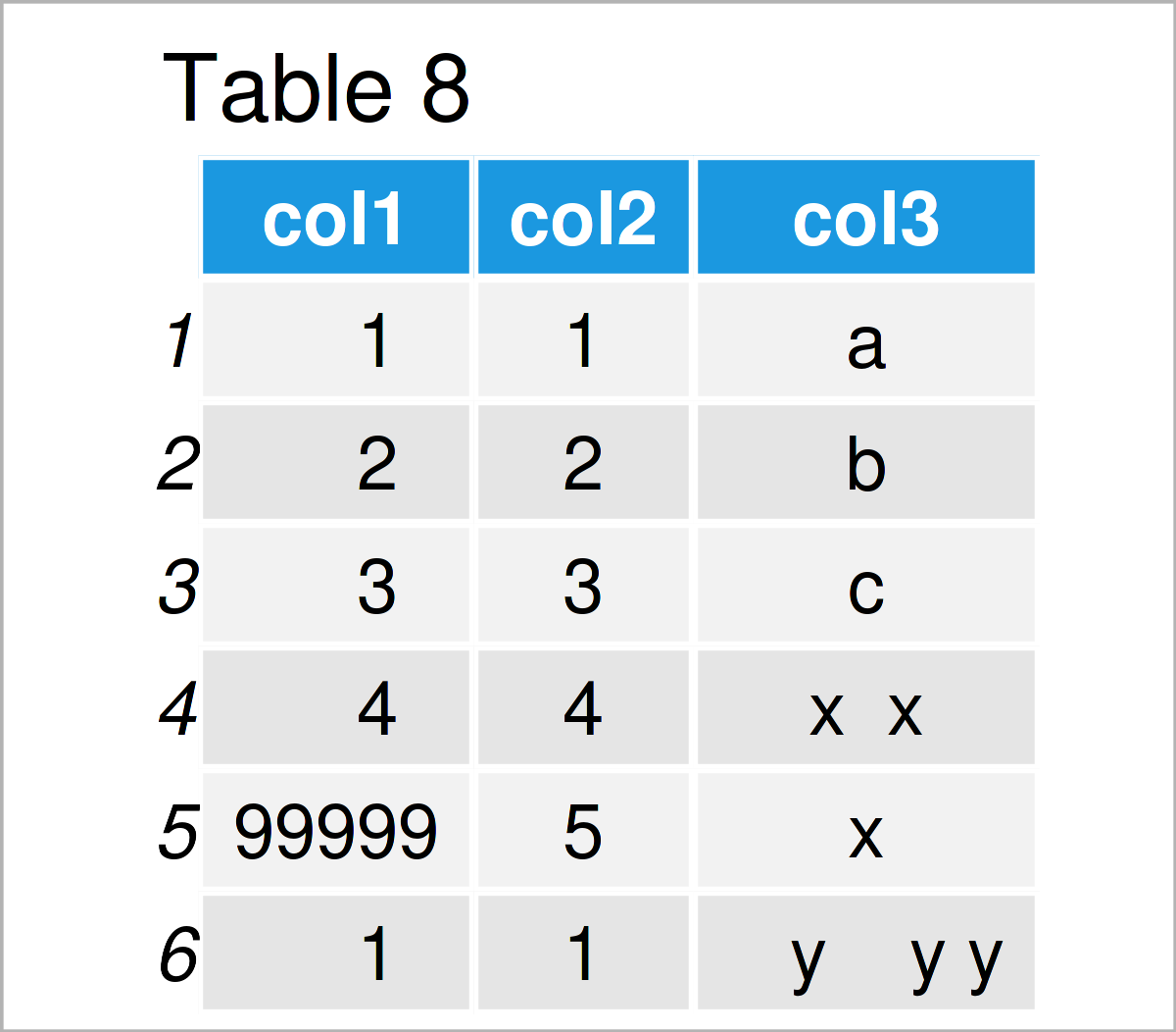
The output of the previous syntax is shown in Table 8: Visually, there’s no difference.

However, if we print the data types of our columns once again, we can see that the first two columns have been changed to the integer class. The character class was retained for the third column.

sapply(data, class)                                       # Print classes of updated columns
#        col1        col2        col3 
#   "integer"   "integer" "character"

Example 7: Detect & Remove Outliers

In Example 7, I’ll demonstrate how to detect and delete outliers.

Please note: Outlier deletion is another very controversial topic. Please verify that it is justified to extract the outliers from your data frame. Please have a look at the outlier removal guidelines here.

However, one method to detect outliers is provided by the boxplot.stats function. The following R code demonstrates how to test for outliers in our data frame column col1:

data$col1[data$col1 %in% boxplot.stats(data$col1)$out]    # Identify outliers in column
# [1] 99999

The previous output has returned one outlier (i.e. the value 99999). This value is obviously much higher than the other values in this column.

Let’s assume that we have confirmed theoretically that the observation containing this outlier should be removed. Then, we can apply the R code below:

data <- data[! data$col1 %in% boxplot.stats(data$col1)$out, ]  # Remove rows with outliers
data                                                      # Print updated data frame

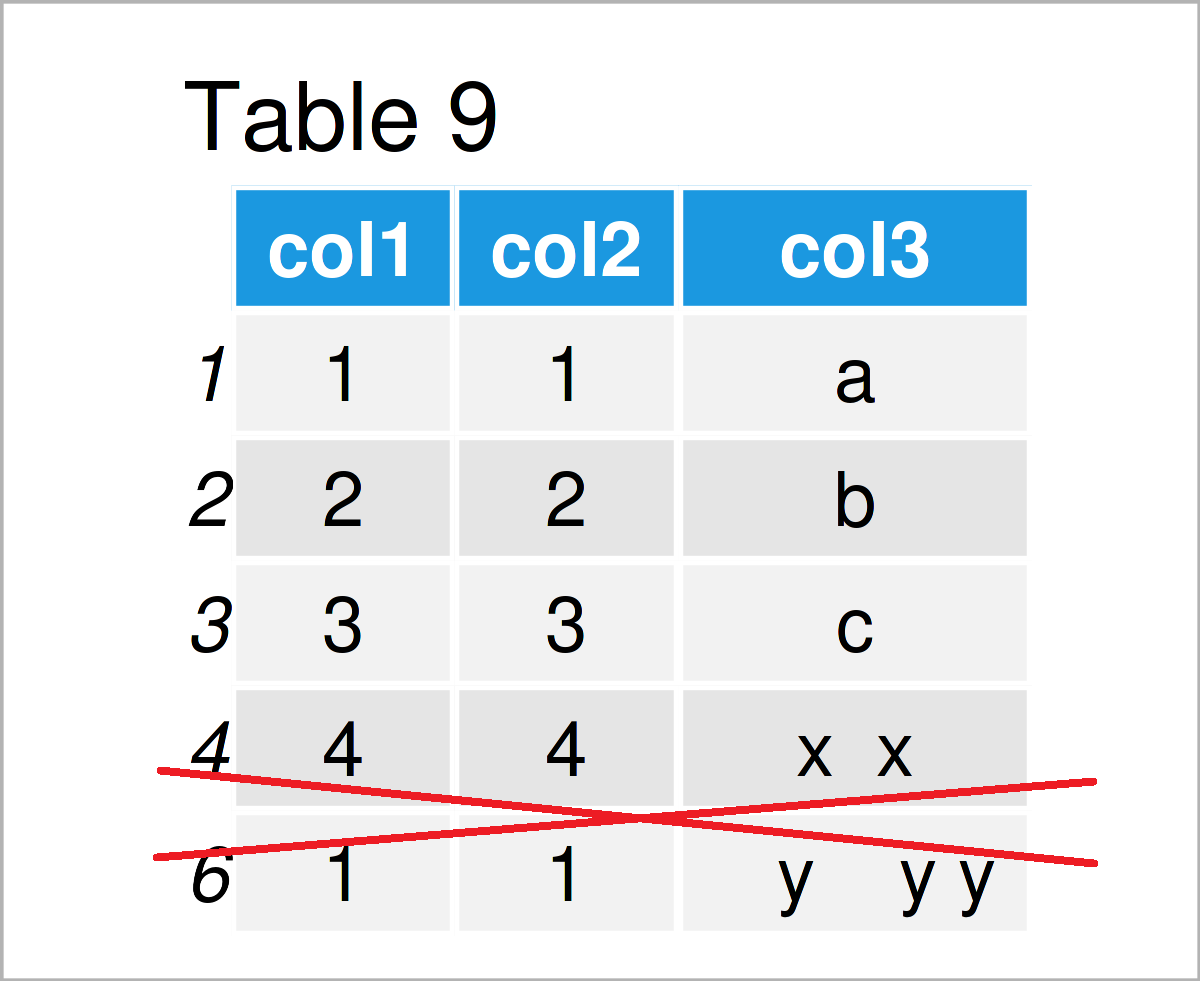
After running the previous R programming syntax the data frame without outlier shown in Table 9 has been created.

Example 8: Remove Spaces in Character Strings

The manipulation of character strings is another important aspect of the data cleaning process.

This example demonstrates how to avoid blank spaces in the character strings of a certain variable.

For this task, we can use the gsub function as demonstrated below:

data$col3 <- gsub(" ", "", data$col3)           # Delete white space in character strings
data                                            # Print updated data frame

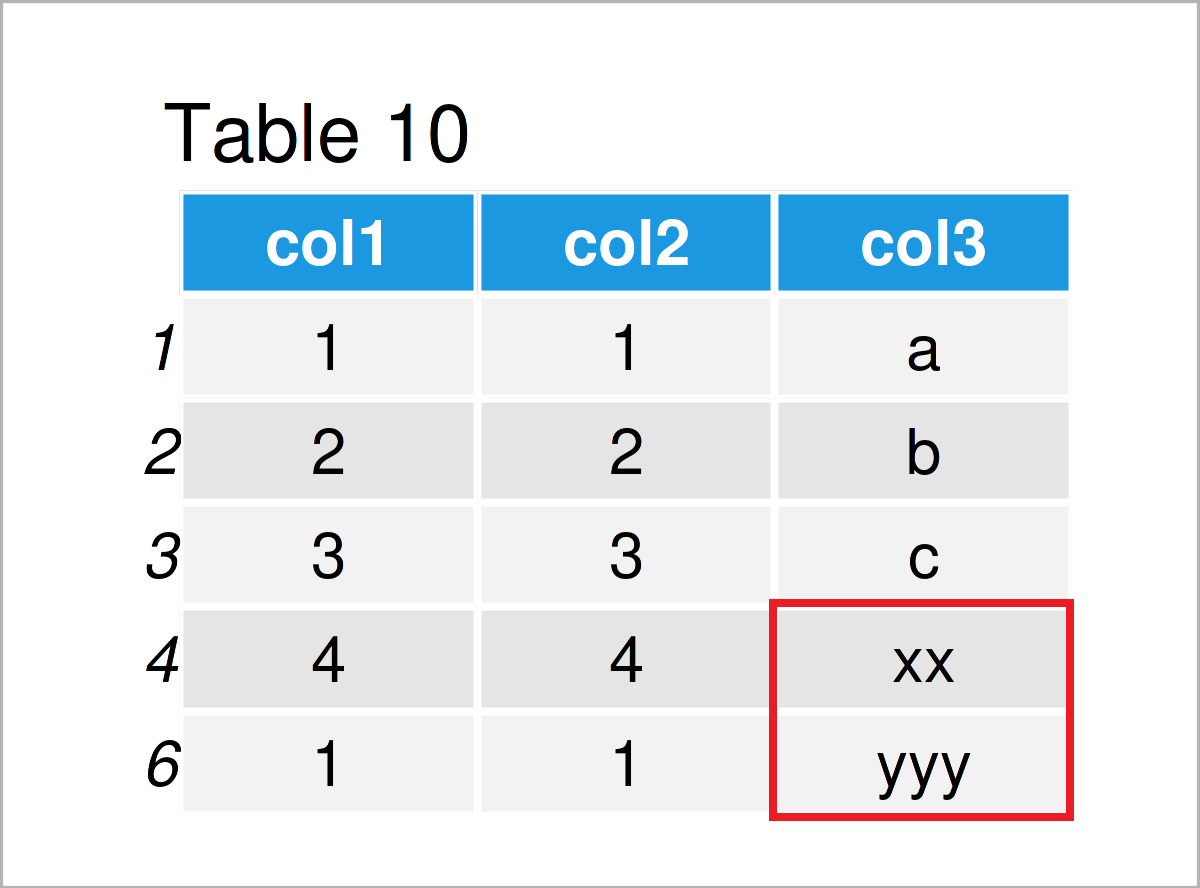
Table 10 shows the output of the previous syntax: All blanks in the column col3 have been dropped and only the actual letters have been kept.

Example 9: Combine Categories

Example 9 shows how to merge certain categories of a categorical variable.

The following R code illustrates how to group the categories “a”, “b”, and “c” in a single category “a”.

Consider the R syntax below:

data$col3[data$col3 %in% c("b", "c")] <- "a"              # Merge categories
data                                                      # Print updated data frame

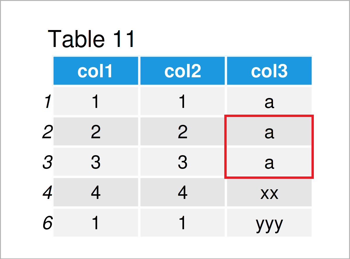
As shown in Table 11, we have created another version of our data frame where the categories “b” and “c” have been replaced by the category “a”.

Video & Further Resources

Note that this tutorial has only shown a brief introduction to different data cleaning techniques.

I have recently released a video on my YouTube channel, which demonstrates the R programming code and the instruction text of this tutorial in some more detail. Please find the video below:

The YouTube video will be added soon.

In addition, you might want to read the related posts to this topic on Statistics Globe.

• Insert Character Pattern at Particular Position of String
• Add Header to Data Frame in R
• Remove Bottom N Rows from Data Frame
• Only Import Selected Columns of Data in R
• Reshape Data Frame from Long to Wide Format
• Replace Specific Characters in String in R
• R Programming Examples

You may also use the search icon on the top-right side of the Statistics Globe menu bar as a cheat sheet, in case you are looking for specific and more detailed advice on a certain topic step-by-step.

Furthermore, I recommend having a look at packages such as dplyr, tidyverse, and stringr. They provide additional functions and commands for the application of data cleaning techniques and are very useful when it comes to the preparation and handling of data frames.

In summary: In this tutorial you have learned how to prepare and clean bad data frames for survey data and other types of data sets in R. In case you have additional questions, kindly let me know in the comments below.