Draw Plot with Two Y-Axes in R (Example)

In this R programming tutorial you’ll learn how to create a plot with two y-axes in Base R.

Table of contents:

Here’s how to do it:

Creation of Example Data

First, we need to create some example data for the plot of this example:

set.seed(25852)                             # Create example data
x <- rnorm(30)
y1 <- x + rnorm(30)
y2 <- x + rnorm(30, 5)

Our example data consists of three numeric vectors: x, y1, and y2.

Now, let’s plot these data!

Example: Create Plot with 2 Axes in R

If we want to draw a plot with two different y-axes, we can use the following R code:

par(mar = c(5, 4, 4, 4) + 0.3)              # Additional space for second y-axis
plot(x, y1, pch = 16, col = 2)              # Create first plot
par(new = TRUE)                             # Add new plot
plot(x, y2, pch = 17, col = 3,              # Create second plot without axes
     axes = FALSE, xlab = "", ylab = "")
axis(side = 4, at = pretty(range(y2)))      # Add second axis
mtext("y2", side = 4, line = 3)             # Add second axis label

plot with two y axes in r

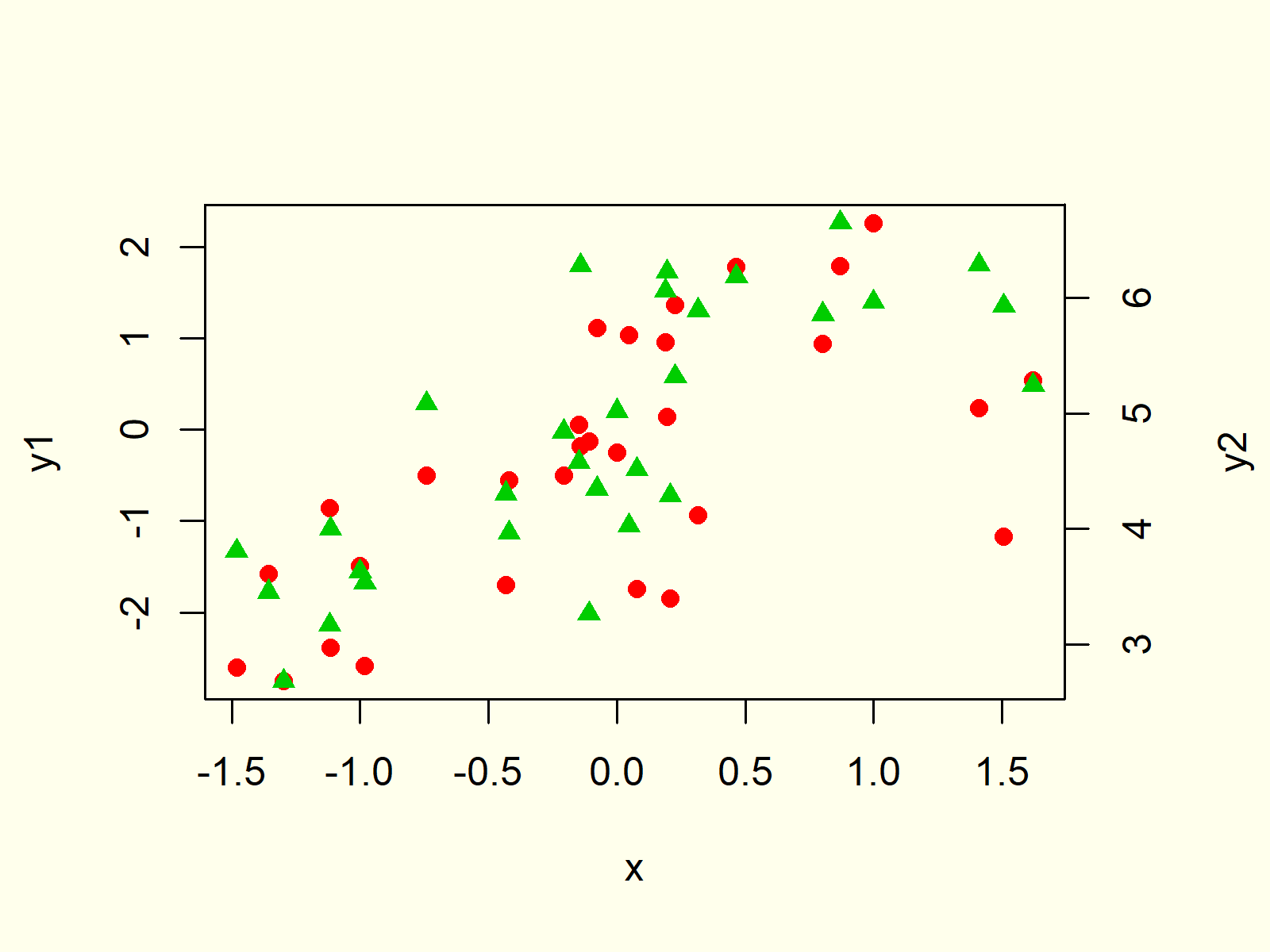
Figure 1: Plot with 2 Y-Axes in R.

Figure 1 is illustrating the output of the previous R syntax. As you can see, we created a scatterplot with two different colors and different y-axis values on the left and right side of the plot.

How did we do that? Let’s deconstruct the code:

par(mar = c(5, 4, 4, 4) + 0.3) – This code defines how much white space should be shown around the plot. It is important to leave enough space for the second y-axis.
plot(x, y1, pch = 16, col = 2) – This code creates the first plot (i.e. the red dots).
par(new = TRUE) – This code specifies that we want to overlay a second plot.
plot(x, y2, pch = 17, col = 3, axes = FALSE, xlab = “”, ylab = “”) – This code draws the second plot (i.e. the green triangles).
axis(side = 4, at = pretty(range(y2))) – This code adds the axis labels on the right side.
mtext(“y2”, side = 4, line = 3) – This code adds the name of the second y-axis (i.e. y2).

Note that this code is adapted from this thread on Stack Overflow. Have a look at this thread for more examples of the plotting of multiple axes.

Also note that we used a scatterplot for this example. However, you may add a secondary axis to many different types of graphics such as boxplots, line charts, histograms, density plots, and so on…

Video, Further Resources & Summary

I have recently released a video on my YouTube channel, which explains the R programming code of this tutorial. You can find the video below:

Please accept YouTube cookies to play this video. By accepting you will be accessing content from YouTube, a service provided by an external third party.

YouTube privacy policy

If you accept this notice, your choice will be saved and the page will refresh.

Furthermore, you might want to have a look at the related tutorials on my homepage:

In summary: This article explained how to add dual axes to a plot in the R programming language. Don’t hesitate to let me know in the comments, in case you have further comments or questions.

18 Comments. Leave new

Morgan
June 12, 2021 6:02 pm

Great code! Thank you! I am having trouble trying to add a legend to this plot since there are two separate plots layered on one another. Would you be able to show how to add a legend to this plot structure?

Reply
- Joachim
  June 14, 2021 6:40 am
  Hey Morgan,
  
  Thank you for the nice comment!
  
  You would have to add the legend at the very end of the code. For example, try to add the following code at the end:
  legend("topleft", legend = c("A", "B"), col = 2:3, pch = 16:17)
  legend("topleft", legend = c("A", "B"), col = 2:3, pch = 16:17)
  Regards
  
  Joachim
  Reply
Maria Alejandra Munoz torres
September 16, 2021 8:01 am

Hi, nice code, How I can add space to not superpose the dot. Thanks

Reply
- Joachim
  September 16, 2021 11:15 am
  Hey Maria,
  
  You may decrease the size of the points and triangles using the cex argument. For instance:
  plot(x, y1, pch = 16, col = 2, cex = 0.5)
  plot(x, y1, pch = 16, col = 2, cex = 0.5)
  Regards
  
  Joachim
  Reply
Maria Alejandra Munoz torres
September 16, 2021 5:37 pm

I couldnt solve adding cex = 0.5 because I am doing a boxplot graph, this is my code:

par(mar = c(5, 4, 4, 4) + 0.5)
boxplot (MOR~ sample1, my_data, pch = 16, col = 2, cex=0.5)
par(new = TRUE)
boxplot(density~sample1, my_data, axes= FALSE, xlab = “”, ylab = “”)
axis(side = 4, line=0, at = pretty(range(density))) # Add second axis
mtext(“density”, side = 4, line = 3)

Reply
- Joachim
  September 17, 2021 5:24 am
  
  Ah, I see. In case of boxplots you would have to use the boxwex argument (e.g. boxwex = 0.5) instead of cex to change the width of the boxes.
  
  Another (likely even better) alternative might be the at argument as explained in Example 8 of this tutorial: https://statisticsglobe.com/boxplot-in-r
  
  Regards
  
  Joachim
  
  Reply
Luis Aviles
October 29, 2021 2:50 am

Hello, I really like your posts!
Is this a way to do this with ggplot?
L.

Reply
- Joachim
  October 29, 2021 5:41 am
  
  Hey Luis,
  
  Thank you for the kind words!
  
  As far as I know, the ggplot2 package restricts the usage of two y-axes. One way to draw two y-axes in a ggplot2 plot is shown here: https://statisticsglobe.com/draw-ggplot2-plot-with-two-y-axes-in-r The resulting plot is not the same as the plot shown in this tutorial though.
  
  Regards,
  Joachim
  
  Reply
Edwin
November 1, 2021 4:12 pm

Hi Joachim,

I am wondering whether is it possible to fit a linear regression with predicted output (yi) and real output (yhati) into this code?

Reply
- Joachim
  November 2, 2021 8:55 am
  
  Hey Edwin,
  
  Have you tried to use the abline function as explained here? https://statisticsglobe.com/abline-function-in-r/#example-6-draw-regression-line-to-plot-using-abline-function
  
  Regards,
  Joachim
  
  Reply
Ben
December 8, 2021 12:29 am

Hi I was wondering if it is possible to put factors on the x-axis? So instead of -1.5, -1.0 etc, what function would you use to put for example “Day 1, Day 2” etc.

Reply
- Joachim
  December 8, 2021 6:55 am
  
  Hey Ben,
  
  Please have a look here: https://statisticsglobe.com/replace-x-axis-values-in-r
  
  Regards,
  Joachim
  
  Reply
Meg
May 24, 2022 7:21 pm

Hello! I am wondering if it is possible to change the ticks on the second y-axis? For example, I would like a range of 1690 to 1700 with ticks spaced apart 1 digit. (1690, 1691, 1692, etc)

Reply
- Joachim
  May 25, 2022 5:50 am
  
  Hi Meg,
  
  You can do that by specifying the at argument within the axis function accordingly. In this example, I have used the pretty function to specify the axis values. However, you can assign basically any value you want to the at argument.
  
  You may also have a look here for more details on the axis function.
  
  Regards,
  Joachim
  
  Reply
Trine Bak
June 17, 2022 8:12 am

Hey
I’m having some problems with adding the right axis. I can add the text “BALF” but the values at the axis dosen’t show.
This is my code:

par(mar=c(4,4,4,4))
boxplot(BALFogELF$ELF~BALFogELF$Study,pch=16,col=2)
par(new=TRUE)
boxplot(BALFogELF$ï..BALF~BALFogELF$Study,pch=17,col=3,axes=TRUE,xlab=””,ylab=””)
axis(side=4,at=pretty(range(BALFogELF$ï..BALF)))
mtext(“BALF”,side=4,line=3)

I hope you can help 🙂

Reply
- Joachim
  June 20, 2022 7:31 am
  
  Hey Trine,
  
  Could you illustrate the structure of the column BALFogELF$ï..BALF? What is returned when you print this column to the console?
  
  Regards,
  Joachim
  
  Reply
Fausto
September 13, 2022 8:50 pm

Thanks for the cool code! Is there any chance to change number facing to the graph? I mean a 180o rotation both numbers and axys name

Reply
- Joachim
  September 19, 2022 11:14 am
  
  Hi Fausto,
  
  Thank you for the kind words, glad you like the code!
  
  I just returned from holidays, so unfortunately, I couldn’t respond to your question earlier. Are you still looking for help?
  
  Regards,
  Joachim
  
  Reply