Listwise Deletion for Missing Data (Is Complete Case Analysis Legit?)

Complete data without any missing values is needed for many kinds of calculations, e.g. regression or correlation analyses. Listwise deletion is used to create such a complete data set.

Many software packages such as R, SAS, Stata or SPSS use listwise deletion as default method, if nothing else is specified. Even though you might not have heard about listwise or casewise deletion yet, you have probably already used it.

In this post I’m going to show you everything you need to know for applying listwise deletion to your own data (Hint: You might not want to use listwise deletion anymore, after reading this article).

Select the topic you are interested in:

Example of Complete Case Analysis for Missing Data in R

In the following, I’m going to show you an example in the statistical programming language R, which illustrates how complete case analysis works.

Consider the following example data:

##### Create some synthetic example data #####
 
set.seed(34567) # Set seed to get a reproducible example
 
N <- 1000 # Sample size
 
y <- rnorm(N) # Outcome/target variable
x1 <- rnorm(N, 10, 5) # First independent/auxiliary variable; This variable is uncorrelated with y
x2 <- y + rnorm(N, 2, 5) # Second independent/auxiliary variable; This variable is correlated with y
x3 <- y + rnorm(N, - 5, 8) # Second independent/auxiliary variable; Also correlated with y
 
data <- round(data.frame(y, x1, x2, x3), 2) # Store data in a data frame
head(data)
 
data$y[rbinom(N, 1, 0.9) == 0] <- NA # 10% missing values in y
data$x1[rbinom(N, 1, 0.8) == 0] <- NA # 20% missing values in x1
head(data)

Table 1: First 6 Rows of Our Synthetic Example Data

As you can see in Table 1, there are missing values (in R displayed as NA) in the target variable Y (response rate 90%) and in the auxiliary variable X1 (response rate 80%). The variables X2 and X3 do not contain any missing values.

This is a typical situation that you may also find in reality. Missing rates of 20 or more percent are nothing special in voluntary surveys. Especially sensitive questions about income, sexual orientation, or age are at risk for high nonresponse rates.

Lately, for instance, I was working on some data about income and living conditions and I was confronted with missing rates in income variables of 10-25%.

But what does that mean for our data analyses? Let’s do a simple example based on our previously created synthetic data with missing values:

##### Exemplifying regression analysis #####
 
model <- lm(y ~., data) # Estimate regression model
summary(model) # Summary of our regression

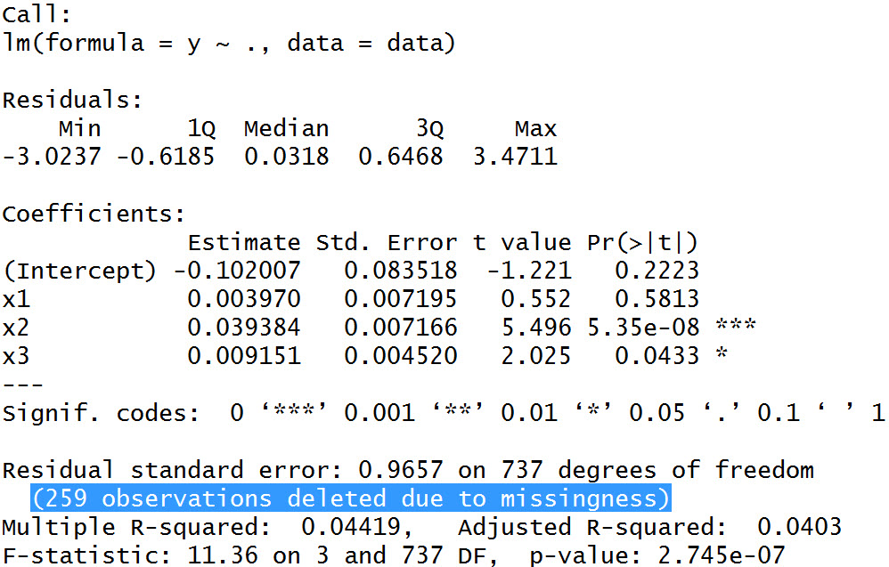
Table 2: Summary Output of Our Regression Analysis

In Table 2, you can see some regular output of a linear regression on our dependent variable Y. The variable X1 does not have a significant impact on Y – no surprise, since we didn’t model any correlation between X1 and Y, when we created our synthetic data.

The variables X2 and X3, in contrast, are highly significant predictors for our target variable Y – again no surprise.

The difference compared to an analysis without missing values can be found in the description of our output: In the description of our regression output in Table 2 you can read the line “259 observations deleted due to missingness“.

Because of listwise deletion, our sample size was shrinked from 1,000 to 741 observations – a loss of more than 25%! That’s like throwing away 259 individuals from our data set in the forefront of our analysis.

Listwise deletion for missing data in R is conducted manually as follows:

##### Listwise deletion by hand #####
 
data_complete_cases <- data[complete.cases(data), ]
dim(data_complete_cases)
 
# [1] 741   4

After conducting casewise deletion with the complete.cases function there are only 741 observations left.

If you execute the previous regression analyses again with our complete data, you will get exactly the same results:

model_complete_cases <- lm(y ~., data_complete_cases) # Estimate regression model
summary(model_complete_cases) # Summary of our regression

In case of regression analysis, R deletes all incomplete observations by default. However, this is not always the case.

If you want to perform a correlation analysis, for example, you will see that R is not automatically deleting incomplete cases. You would have to do a listwise deletion manually:

##### Correlation analysis with and without listwise deletion #####
 
cor(data$y, data$x1) # NA --> The function cor() is not deleting missing observations by default
cor(data_complete_cases$y, data_complete_cases$x1) # Correlation of complete data

With complete case files such as data_complete_cases you could do every analysis you want without getting any problems.

Is Complete Case Analysis Legit?

Although the simplicity of complete case analysis is a major advantage, listwise deletion causes big problems in many missing data situations.

There are two major reasons, why casewise deletion might be problematic:

1. The sample size is reduced
2. The reasons for missing values might not be random

Let’s have a closer look at these two problems!

The first problem – a smaller sample size – was already illustrated in the previous complete case study examples. As you have seen, more than 25% of our data was deleted. Obviously that’s a huge loss for our statistical data analysis.

Plain and simple: A smaller sample size leads to less statistical power of our analyses.

The second problem – the randomness of our missing data – might be less intuitive and is therefore often neglected in practice.

In reality, however, the non-randomness of missing data may result in biased estimates and hence in wrong conclusions of your complete case analysis.

The randomness of your missing values, i.e. the missing mechanism, is separated into three different types: Missing Completely At Random (MCAR), Missing At Random (MAR) und Missing Not At Random (MNAR) (Little und Rubin, 2002).

If your missings are MCAR, listwise deletion is less problematic. If your missing values are MAR or MNAR, your complete case study is likely to be biased.

Let’s check our example from above:

##### Graphic for missing and non-missing values #####
 
plot(density(y[!is.na(data$y)]), xlab = "y", main = "Observed and Missing Values of Y")
points(density(y[is.na(data$y)]), type = "l", col = 2)
legend("topleft", c("Observed Values", "Missing Values"), lty = 1, col = 1:2)

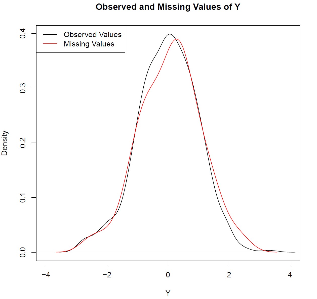
Graphic 1: Observed and Missing Values of Y

As you can see based on Graphic 1, there are only slight differences between the densities of observed and missing values.

A Kolmogorov-Smirnov Test confirms what we already saw graphically: The differences of our observed and unobserved values are not significant.

##### Kolmogorov–Smirnov test between missing and non-missing values #####
 
ks.test(y[!is.na(data$y)], y[is.na(data$y)])

Table 3: Kolmogorov-Smirnov Test of Observed and Missing Data

Be aware that we were able to inspect the missing mechanisms with these statistical tests, since we created the data ourselves. In reality we would not be able to perform such tests and therefore we would need to rely on theoretical assumptions about the randomness of our incomplete data.

However, it is in general very rare in statistics that missing data is MCAR! In most cases you should try to use more sophisticated methods such as missing data imputation to take the missing data and the structure of the missingness into account.

Note: Not all imputation methods reduce bias. In fact, some methods (e.g. mean imputation or a replace of missing data by zero) even increase bias. Learn here, which method is appropriate for your specific database.

However, let’s see what happens, if we have some systematic structure in our missing values (much more realistic). For illustration, consider the following example data:

set.seed(987654321) # Set seed to get a reproducible example
 
N <- 5000 # Increased sample size, to make the effect more visible
 
y <- rnorm(N) # Our outcome/target variable. No missing values yet
x <- 2 * y + rnorm(N, 10, 5) # Independent/auxiliary variable; This variable is correlated with y
 
resp_prop <- x + rnorm(N, 10, 5) # Systematic influence of x on the missingness in y.
                                 # Observations with lower values in x have a
                                 # lower response propensity in y
resp_prop[resp_prop < mean(resp_prop)] <- NA # Approximately 50% systematic missing values in y

Now let’s graphically check how observed and missing values of Y are distributed.

par(mfrow = c(1, 2)) # 2 plots in one graphic
 
plot(density(y[!is.na(resp_prop)]),  # Observed values in black
     xlim = c(- 4, 4), ylim = c(0, 0.48), 
     xlab = "Y", main = "Observed and Missing Values of Y")
points(density(y[is.na(resp_prop)]), type = "l", col = 2) # Missing data in red
legend("topleft", c("Observed Values", "Missing Values"), lty = 1, col = 1:2)
 
plot(x[!is.na(resp_prop)], y[!is.na(resp_prop)],  # Observed values in black
     xlim = c(- 10, 30), ylim = c(- 4, 5), 
     xlab = "X", ylab = "Y", main = "Correlation Plot of X and Y")
points(x[is.na(resp_prop)], y[is.na(resp_prop)], col = 2) # Missing data in red
abline(h = mean(y), lwd = 2, col = "deepskyblue", lty = "dashed") # True mean (observed & missing combined)
abline(h = mean(y[!is.na(resp_prop)]), lwd = 2) # Mean of observed values
abline(h = mean(y[is.na(resp_prop)]), lwd = 2, col = 2) # Mean of observed values
legend("topleft", 
       c("Observed Values", "Missing Values", "Observed Values Mean", "Missing Values Mean", "True Mean"),
       pch = c(1, 1, NA, NA, NA), 
       lwd = c(NA, NA, 1, 1, 1), 
       col = c(1, 2, 1, 2, "deepskyblue"),
       lty = c("", "", "solid", "solid", "dashed"))

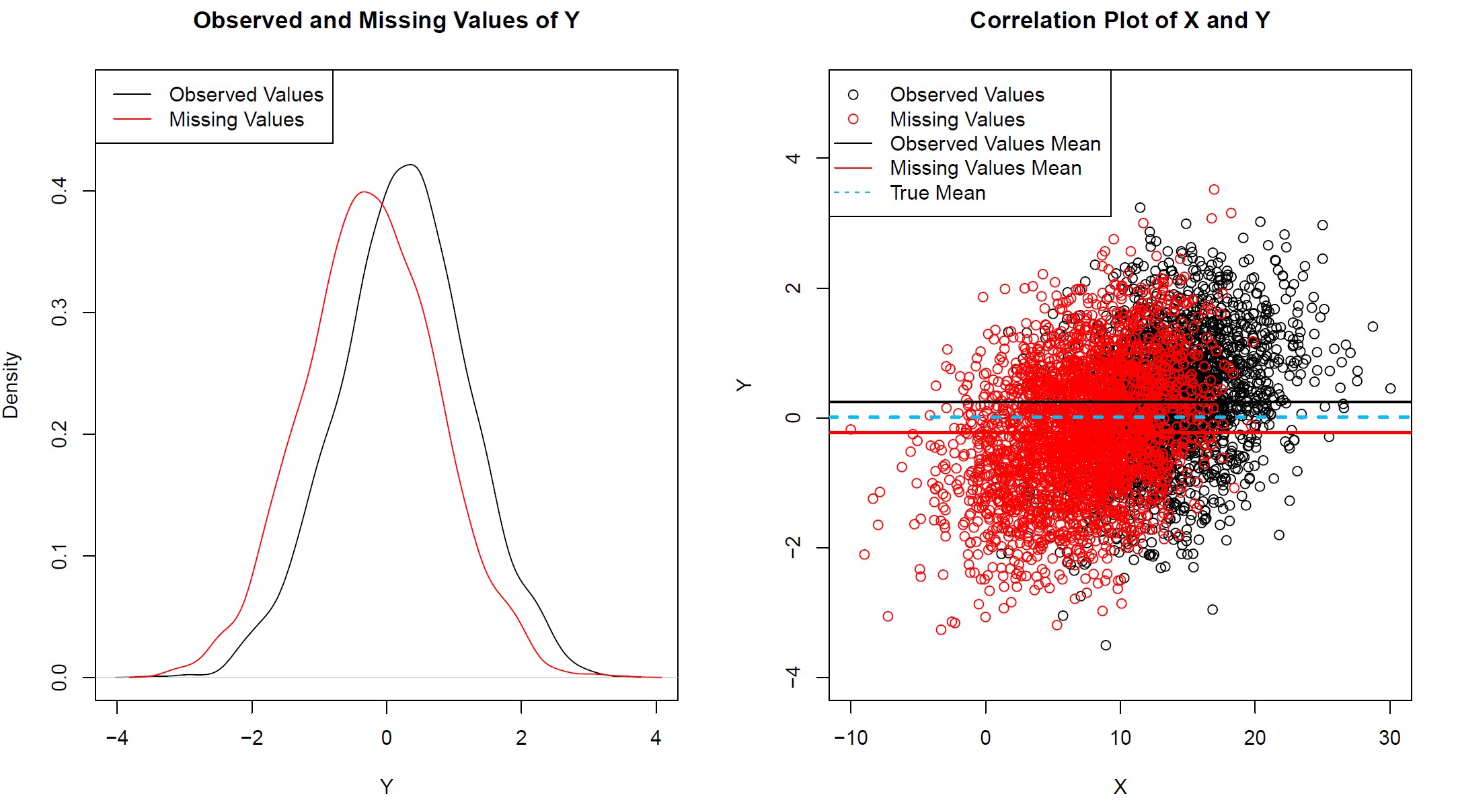
Graphic 2: Observed and Missing Values of Y with Systematic Response Structure

As shown in Graphic 2 in the left pane, the densities of observed and missing values differ. Complete cases seem to be higher on average.

A correlation plot of X and Y is illustrated in the right pane. As modeled before, when we created the synthetic data, there is a positive correlation between X and Y.

However, we can also see that the mean of Y differs between the observed and the missing values. The mean of the missing data, illustrated by the red straight line, indicate a slightly lower value for observations with missingness in Y.

If we would perform a complete case analysis, we would therefore overestimate the mean of Y. Not really the result we would hope to see!

##### Mean of observed and missing values #####
 
round(mean(y[!is.na(resp_prop)]), 2) # Observed values have a mean of 0.24
round(mean(y[is.na(resp_prop)]), 2) # Missing values have a mean of - 0.23

This graphical impression is confirmed by a Kolmogorov-Smirnov Test:

##### Kolmogorov–Smirnov test of missing and non-missing values – systematic missingness #####
 
ks.test(y[!is.na(data$y)], y[is.na(data$y)])

The p-value of the Kolmogorov-Smirnov Test is significant – our missing values are significantly different to our observed data.

So, in order to answer our question “Is Complete Case Analysis Legit?” in short:

• If Problem 2) does NOT occur, our complete case analysis for missing data will have less statistical power, but it will be legit.
• If Problem 2) does occur, we should definitely implement some more advanced methods than listwise deletion to deal with our missing data!

Listwise Deletion in SPSS

Are you not familiar with the programming language R? Don’t worry! There are many other software programs available that can find incomplete rows in your data and perform casewise deletion.

In the following video, the speaker Jason of the YouTube channel SPSSisFun compares three different options for dealing with missing data in SPSS: listwise deletion vs. pairwise deletion vs. mean imputation.

Conclusion

The big advantage of listiwse deletion is that it is easy to understand and to implement. In fact, it is the default method in many statistical software such as R or SPSS.

However, casewise deletion often leads to bias in survey estimates and even if this is not the case, we throw away much valuable information, if listiwse deletion is applied.

More sophisticated methods, e.g. missing data imputation, can be used to replace missings with new values in order to improve data analyses (Allison, 2002).

In short: Listwise deletion is almost never the best choice!

Any Comments or Questions?

I showed you everything I know about listwise deletion.

Now it’s your turn!

Have you also experienced any problems with complete case analyses? Which methods are you using to deal with incomplete data? Do you have any further questions about listwise deletion?

Scroll down and let me know in the comments!

References

Allison, P. D. (2002). Missing data: Quantitative applications in the social sciences. SAGE Publications.

Little, R. J. A. and Rubin, D. B., editors (2002). Statistical Analysis with Missing Data. Wiley-Blackwell.

Appendix

Do you want to know how I created the header graph of this page? Here’s the code!

The graphic shows what happens when listwise deletion is applied – Bias goes up; Sample size goes down.

set.seed(845346) # Set seed to create a reproducible graphic
 
x1 <- sort(runif(50, 0, 100)) * (- 1) # Sample size reduction
x2 <- sort(runif(50, 0, 100)) * 0.75 - 100 # Bias incresement
 
par(bg = "#353436") # Black background of graphic
 
plot(x1, # Plot sample size reduction
     type = "l", 
     lwd = 3,
     col = "#1b98e0",
     xlim = c(0, 60), ylim = c(- 120, 0), 
     xlab = "", ylab = "",
     xaxt = "n", yaxt = "n")
 
abline(v = seq(0, 60, by = 5), col = "steelblue4", lty = 2) # Put some vertical lines on plot
abline(h = seq(- 120, 0, by = 10), col = "steelblue4", lty = 2) # Put some horizontal lines on plot
 
lines(x1, # Plot sample size reduction again in order to verlap the dashed lines
      lwd = 3,
      col = "#1b98e0")
 
lines(x2, # Plot the increase in bias
      lwd = 3, 
      col = "brown1")
 
arrows(c(9, 19, 29, 39, 49), x1[c(9, 19, 29, 39, 49)], # Draw arrows for the reduced sample size
       c(10, 20, 30, 40, 50), x1[c(10, 20, 30, 40, 50)],
       lwd = 3, col = "#1b98e0")
 
arrows(c(9, 19, 29, 39, 49), x2[c(9, 19, 29, 39, 49)], # Draw arrows for the increased bias
       c(10, 20, 30, 40, 50), x2[c(10, 20, 30, 40, 50)],
       lwd = 3, col = "brown1")
 
text(25.1, - 40.3, "Sample Size", cex = 2, col = "#1b98e0") # Put some text on the plot
text(31.5, - 54, "Bias", cex = 2, col = "brown1")