Divide Legend of ggplot2 Plot in R (Example)

On this page you’ll learn how to split a ggplot2 legend into several parts in the R programming language.

The tutorial consists of the following information:

You’re here for the answer, so let’s get straight to the example!

Example Data, Packages & Default Graphic

The following data is used as basement for this R tutorial:

data <- data.frame(x = 20:15,                          # Create example data frame
                   y = 3:8,
                   group = LETTERS[1:6])
data                                                   # Show example data frame

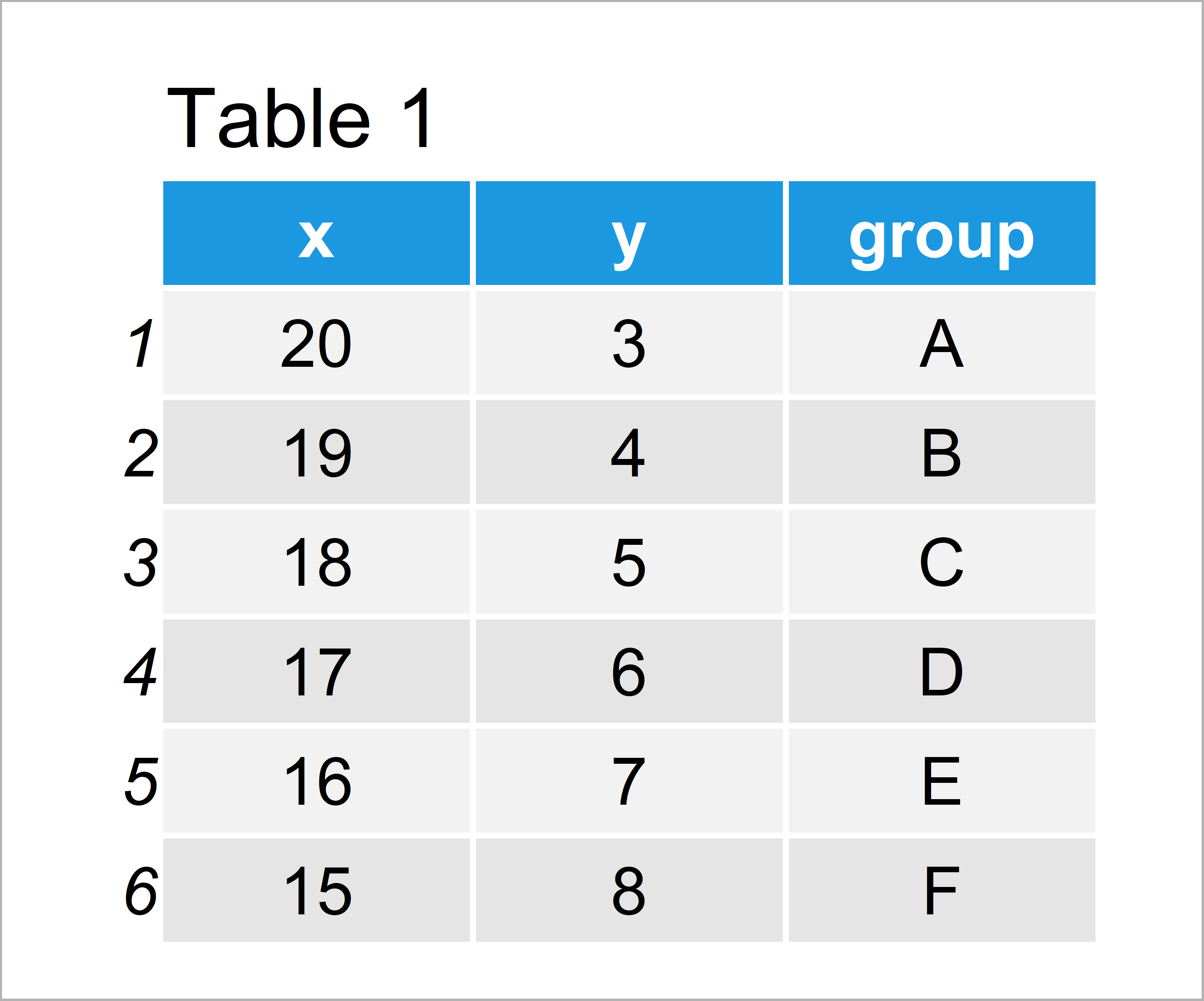
As you can see based on Table 1, our example data is a data frame containing six rows and three columns. The variables x and y contain numeric values and the variable group consists of the corresponding groups.

For the examples of this tutorial, we’ll also have to install and load the ggplot2 package:

install.packages("ggplot2")                            # Install ggplot2 package
library("ggplot2")                                     # Load ggplot2 package

Now, we can draw our data with a single legend as shown below:

ggp <- ggplot(data, aes(x,                             # Creating ggplot2 plot
                        y,
                        color = group)) +
  geom_point(size = 5)
ggp                                                    # Drawing ggplot2 plot

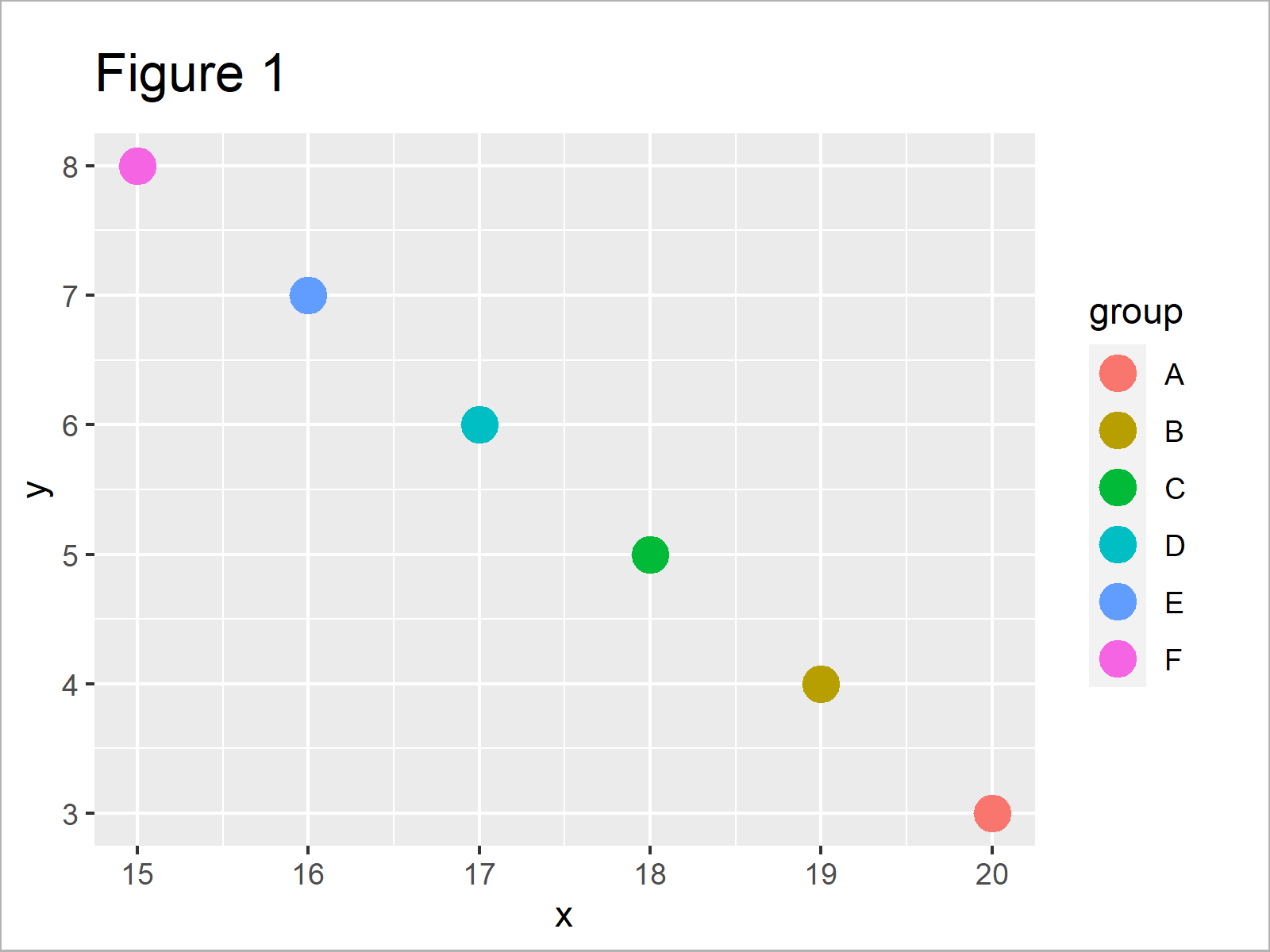
As shown in Figure 1, we have plotted a ggplot2 scatterplot with a single legend by executing the previous R syntax.

Example: Split ggplot2 Legend into Multiple Parts

In this example, I’ll illustrate how to divide the elements of a ggplot2 legend into multiple legends.

For this task, we first have to install and load two additional packages: gridExtra and cowplot.

install.packages("gridExtra")                          # Install & load gridExtra package
library("gridExtra")

install.packages("cowplot")                            # Install & load cowplot
library("cowplot")

As next step, we have to create a data frame subset containing the groups of our first legend:

data_split_1 <- data[data$group %in% c("A", "B"), ]    # Create first data frame subset
data_split_1                                           # Print data frame subset

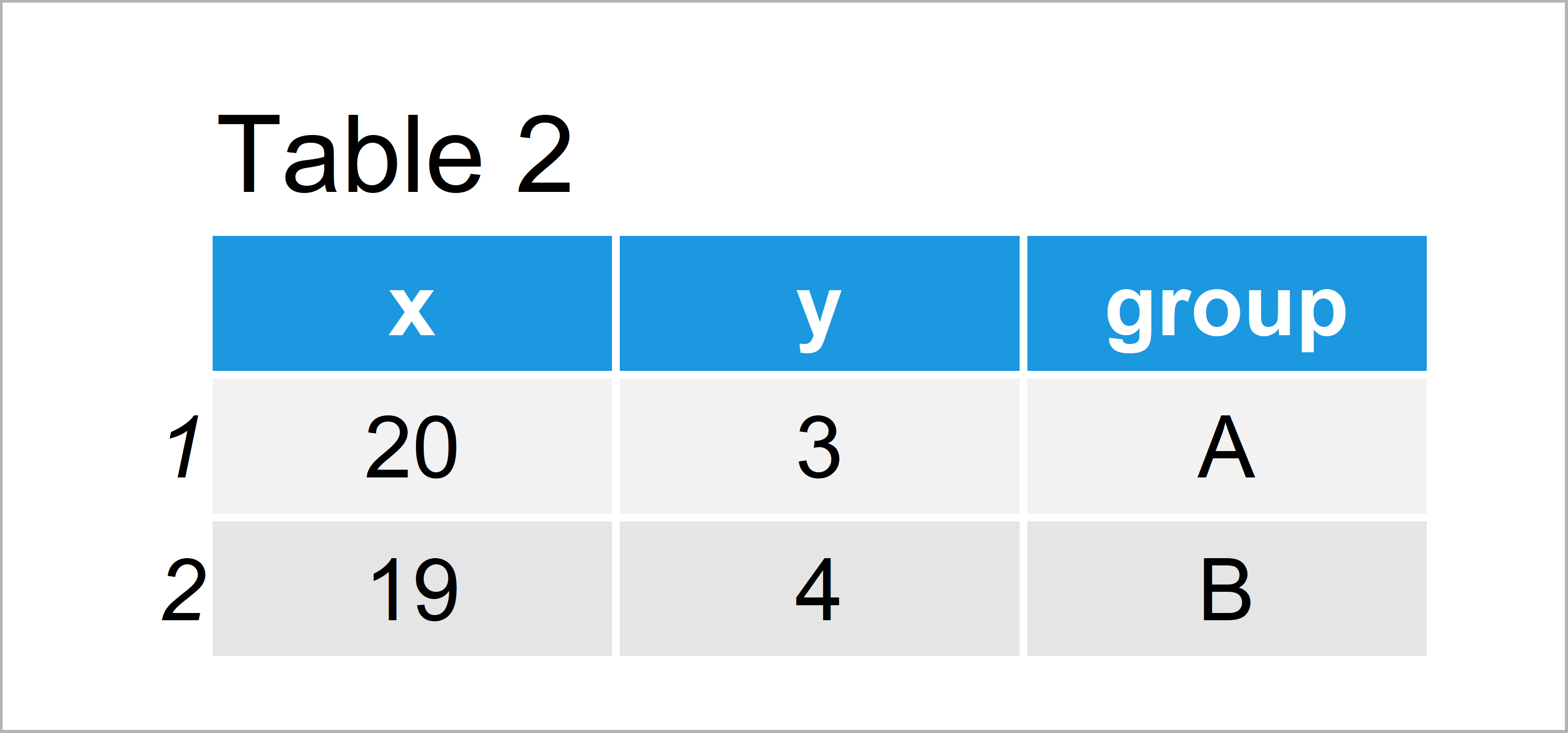
As shown in Table 2, the previous code has created a subset of our example data containing only the groups A and B.

Now, we can create a plot object based on the subset that we have just created:

ggp_split_1 <- ggplot(data_split_1,                    # Create ggplot2 plot of first subset
                      aes(x,
                          y,
                          color = group)) +
  geom_point(size = 5) +
  scale_color_manual(values = 1:2) +
  labs(color = "Legend No. 1")
ggp_split_1                                            # Draw ggplot2 plot of first subset

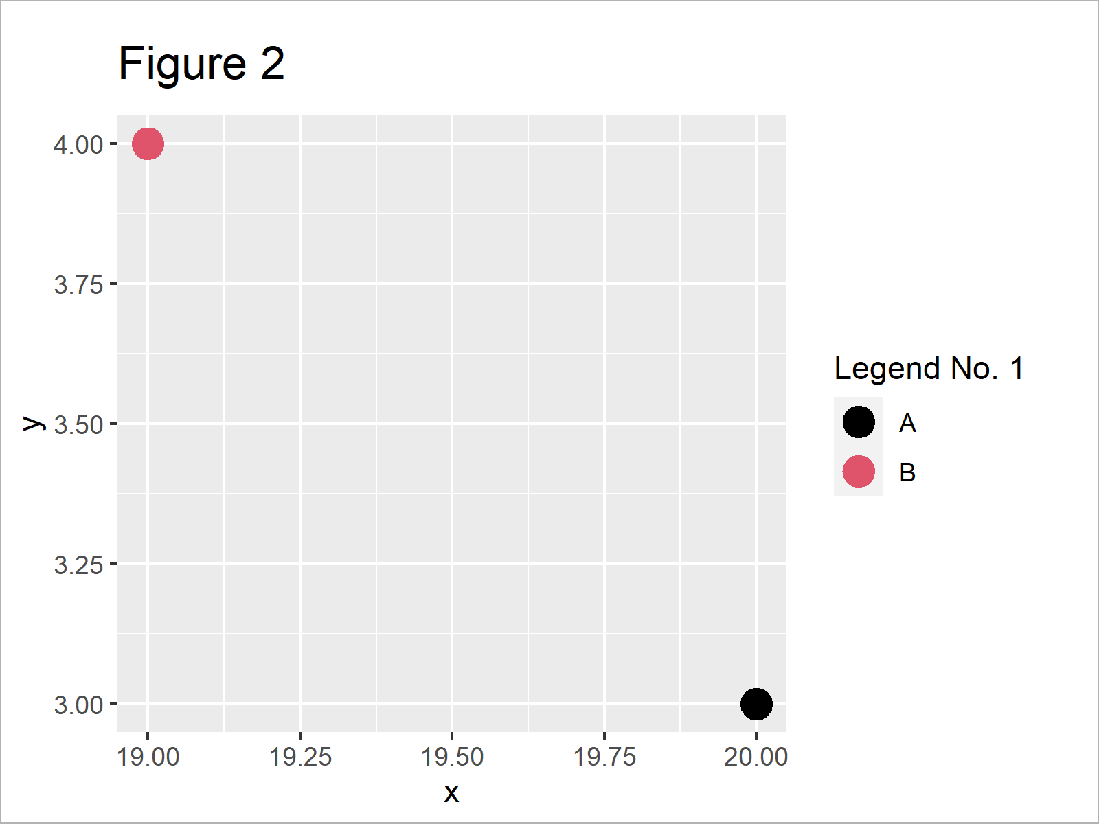
As shown in Figure 2, we have created a plot object with a legend that shows only the groups A and B using the previous R programming code.

Next, we can use the get_legend function of the cowplot package to extract the legend of the previously created plot:

ggp_legend_split_1 <- get_legend(ggp_split_1)          # Extract legend of first subset

The first legend is basically done. Now, we have to repeat this process for the second legend (or for all legends that we want to add to our plot).

Create a subset for the second legend…

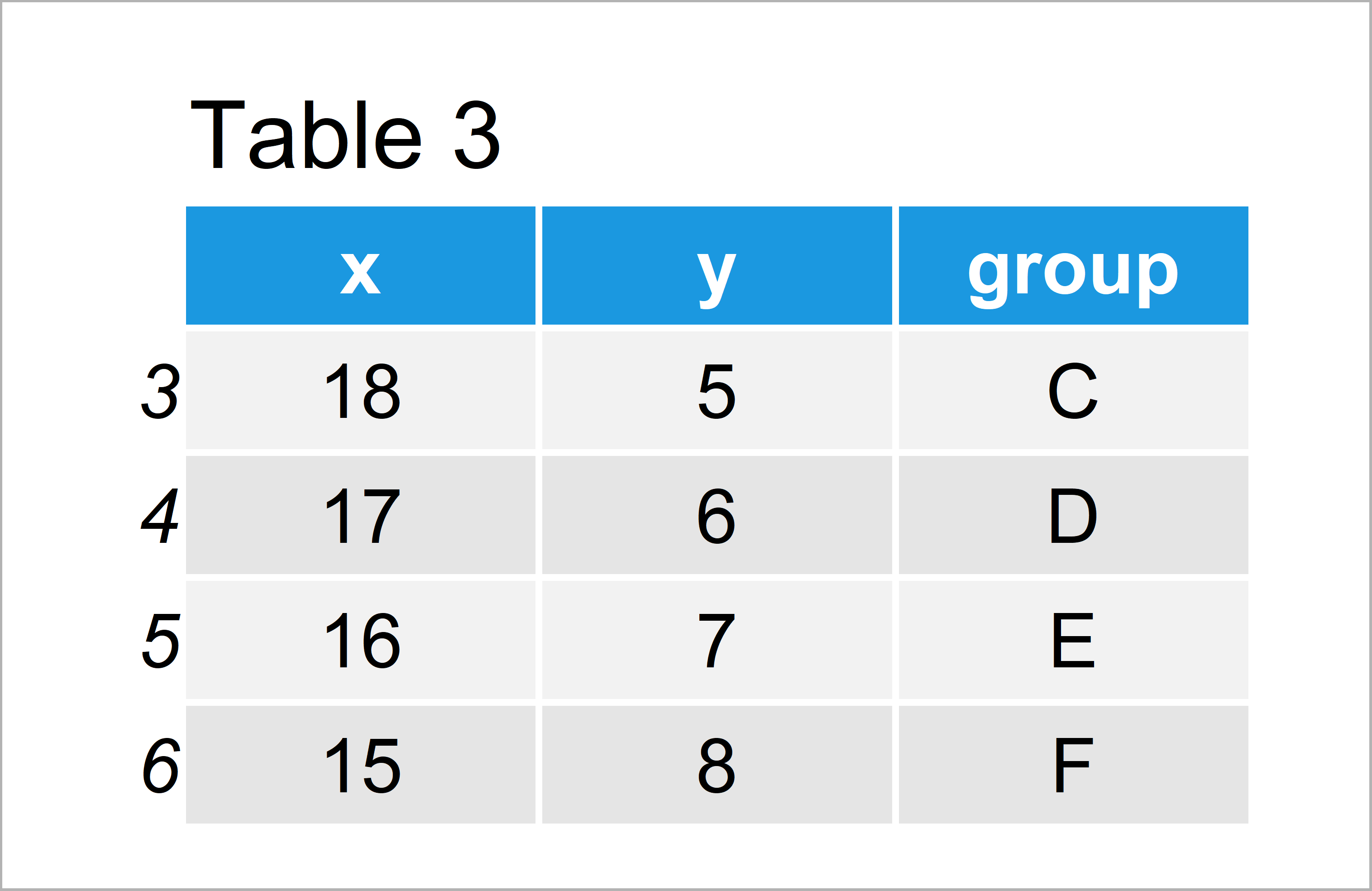
data_split_2 <- data[! data$group %in% c("A", "B"), ]  # Create second data frame subset
data_split_2                                           # Print data frame subset

…create a plot based on this subset…

ggp_split_2 <- ggplot(data_split_2,                    # Create ggplot2 plot of second subset
                      aes(x,
                          y,
                          color = group)) +
  geom_point(size = 5) +
  scale_color_manual(values = 3:6) +
  labs(color = "Legend No. 2")
ggp_split_2                                            # Draw ggplot2 plot of second subset

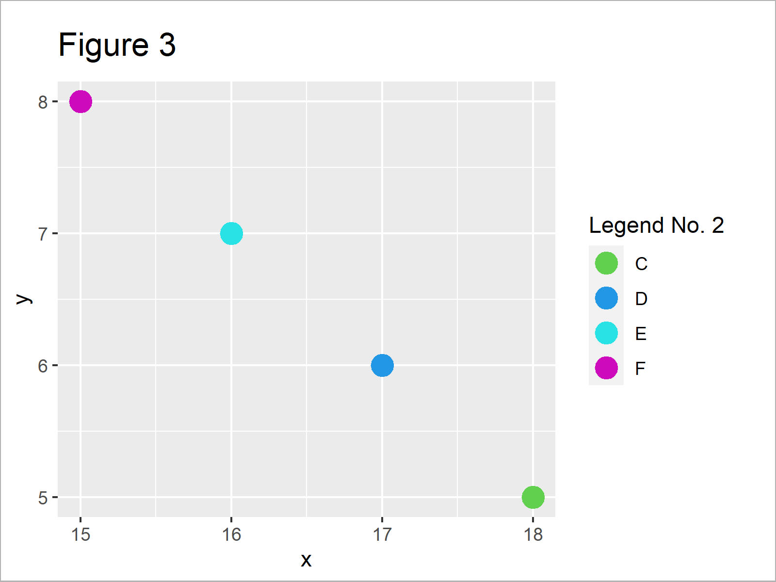
…and extract the legend from this plot:

ggp_legend_split_2 <- get_legend(ggp_split_2)          # Extract legend of second subset

In the next step, we have to create a ggplot2 graphic containing all our data, but without a legend. For this, we have to set the legend.position argument within the theme function to “none”:

ggp_no_legend <- ggplot(data,                          # Create ggplot2 plot without legend
                        aes(x,
                            y,
                            color = group)) +
  geom_point(size = 5) +
  scale_color_manual(values = 1:6) +
  theme(legend.position = "none")
ggp_no_legend                                          # Draw ggplot2 plot without legend

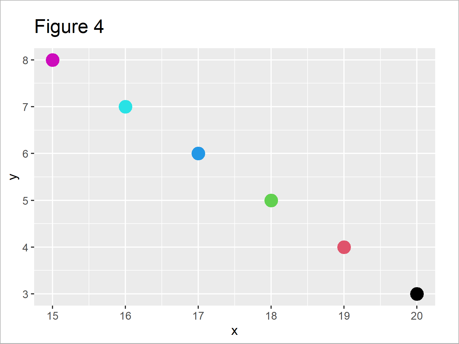
As shown in Figure 4, the previous R syntax has drawn our data to a ggplot2 plot without legend.

Finally, we can combine all plot objects that we have created before in a grid of plots using the grid.arrange function:

grid.arrange(ggp_legend_split_1,                       # Draw ggplot2 plot with two legends
             ggp_no_legend,
             ggp_legend_split_2,
             ncol = 3)

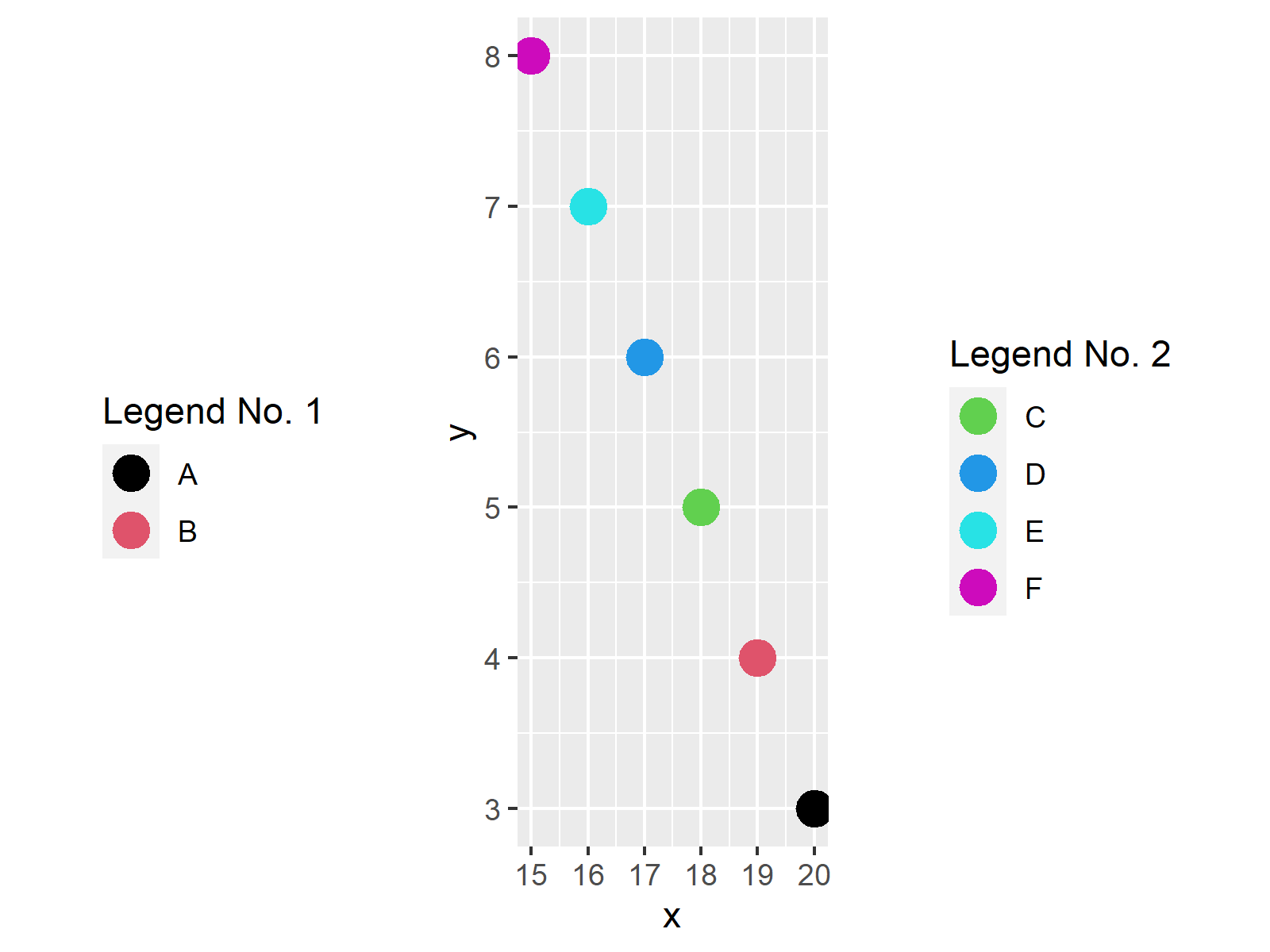
Figure 5 shows our final output: A ggplot2 graphic with two legends.

Note that we could arrange our grid in basically any way we want. Whether you want to draw the legends on the left and right side of the plot (as shown in this example), or at the bottom and top is up to you.

Also note that we could apply the same kind of R code to other types of graphics such as barcharts, histograms, density plots, boxplots, and so on…

Video & Further Resources

In case you need more info on the content of this article, I recommend having a look at the following video which I have published on my YouTube channel. In the video, I explain the R programming syntax of this article:

Furthermore, you might want to read some of the related articles of this website. You can find a selection of tutorials about ggplot2 below:

• Set Legend Alpha of ggplot2 Plot
• Remove Legend Title from ggplot2 Plot in R
• Change Display Order of ggplot2 Plot Legend
• Change Legend Labels of ggplot2 Plot
• Drawing Plots in R
• R Programming Overview

To summarize: In this R programming tutorial you have learned how to divide a ggplot2 legend into multiple parts. Don’t hesitate to let me know in the comments section below, in case you have additional questions and/or comments.