uniroot Function in R (Example)

In this article you’ll learn how to find a one dimensional root using the uniroot function in R programming.

The article consists of the following information:

With that, let’s jump right to the example.

Introduction of Example Function

We’ll use the following function as basement for this R tutorial:

my_fun <- function(x) {               # Create example function
  x^4 - 5000 * x^2 + 30000 * x
}

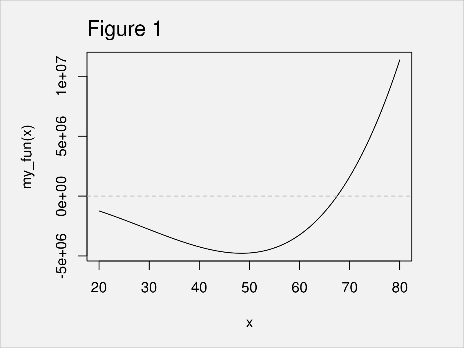
As next step, we can draw our function curve to a plot:

curve(expr = my_fun,                  # Draw function in plot
      from = 20,
      to = 80)
abline(h = 0,
       lty = "dashed",
       col = "gray")

In Figure 1 you can see that we have plotted our function ranging from 20 to 80. As you can see, there is a root within this area.

Example: Find One Dimensional Root of Function Curve Using uniroot()

In this example, I’ll illustrate how to apply the uniroot function to find a root (i.e. zero) within a certain interval.

We can use the uniroot command as shown below:

uniroot_out <- uniroot(f = my_fun,    # Find root
                       interval = c(20, 80))
uniroot_out                           # Output of uniroot function
# $root
# [1] 67.49459
# 
# $f.root
# [1] 0.007518359
# 
# $iter
# [1] 8
# 
# $init.it
# [1] NA
# 
# $estim.prec
# [1] 6.103516e-05

The previous output of the RStudio console shows a list with five different components:

1. root gives the location of the root point.
2. f.root gives the value of the function evaluated at the root point.
3. iter gives the number of iterations used.
4. estim.prec gives an approximate estimated precision for the root point.

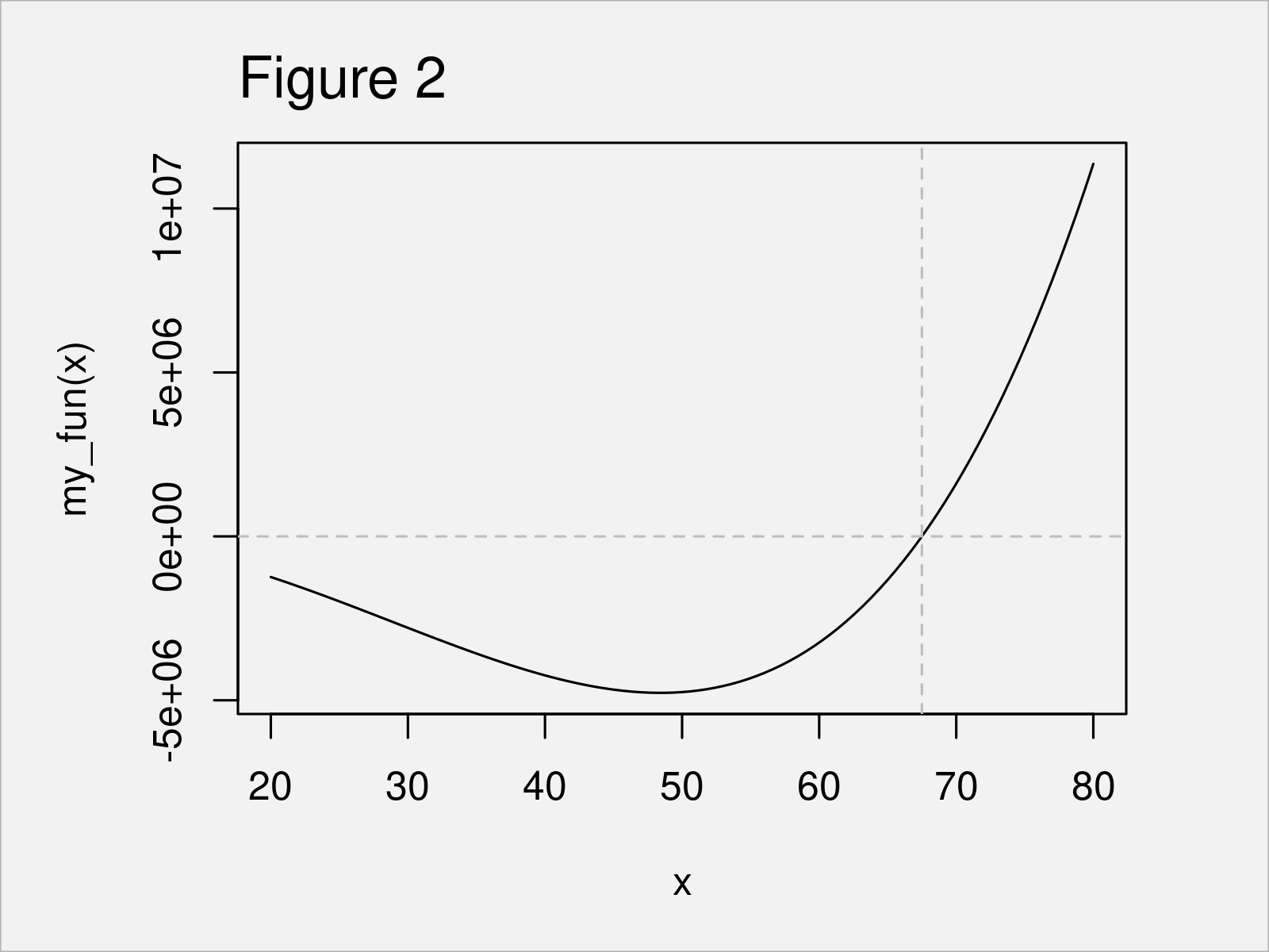
In our example, we are interested in the root value. We can extract this value using the $ operator (i.e. uniroot_out$root). As you can see, the root of our function curve is at the value 67.49459.

We can also visualize this root in our function plot:

curve(expr = my_fun,                  # Add line to function plot
      from = 20,
      to = 80)
abline(h = 0,
       lty = "dashed",
       col = "gray")
abline(v = uniroot_out$root,
       lty = "dashed",
       col = "gray")

After executing the previous R code the function curve plot shown in Figure 2 has been created. The dashed lines indicate the position of the one dimensional root.

Video & Further Resources

I have recently published a video on my YouTube channel, which shows the R codes of this article. You can find the video below:

Furthermore, you could have a look at the other articles on this website. I have published numerous tutorials that are related to the application of the uniroot function already.

• Draw Plot of Function Curve in R
• Draw Multiple Function Curves to Same Plot
• Square Root in R
• Calculate (Root) Mean Squared Error
• Built-in R Commands
• All R Programming Examples

In summary: You have learned in this article how to apply the uniroot function in R. Let me know in the comments below, if you have further comments or questions.