data.table vs. data.frame in R (2 Examples)

In this R tutorial, you’ll learn some differences between a data.table and a data.frame object.

The message in short: Always use data.table instead of data.frame! Data.table is handy, has an intuitive, easy-to-read syntax, and is the object type of choice, especially for large datasets. We illustrate this with two examples.

Make sure to also take a look at our blog post with general information about data.table here. Furthermore, we recommend you this post, which nicely focuses on the use of data.table for big data in R, including data.table commands for efficient loading and saving of data.

Table of contents:

Sound good? Let’s start right away…

Example Data & Software Packages

If we want to use the functions of the data.table package, we first have to install and load data.table. Data.frames, on the other hand, are built-in and can be used without loading an additional package. For our examples and illustrations, we furthermore need to install and load the dplyr and rbenchmark packages.

install.packages("data.table")                      # Install data.table package
library("data.table")                               # Load data.table package
 
install.packages("dplyr")                           # Install dplyr package
library("dplyr")                                    # Load dplyr package
 
install.packages("rbenchmark")                      # Install rbenchmark package
library("rbenchmark")                               # Load rbenchmark package

Let’s construct some example data in R:

set.seed(8)                                         # Set seed for reproducible results
N <- 90000                                          # Number of observations to generate
DF1 <- data.frame(A = rnorm(N),                     # Generate data.frame
                  B = rpois(N, 5),
                  C = sample(letters[1:5], N/5, replace = TRUE))
DT1 <- data.table(DF1)                              # Define a data.table with the same information as DF1
head(DT1)                                           # Print head of data

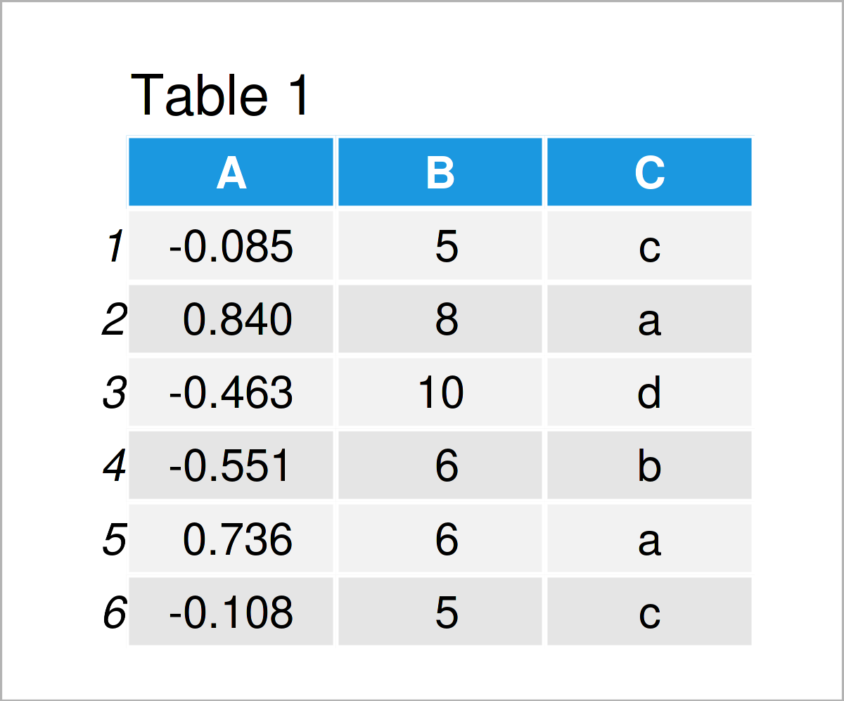
Table 1 shows that our exemplifying data consists of three columns. The variable A is numerical, the variable B is an integer, and the variable C has the character data type. We have the same information in data.frame DF1 and data.table DT1, only their classes differ. You can furthermore see that it is easy to transform a data.frame into a data.table and vice versa.

Example 1: Syntax

The following R programming syntax demonstrates how the syntax between data.frame and data.table objects differs. For that, we demonstrate hoe to calculate group means of a variable for chosen data rows in different ways.

First, we use the piping language of dplyr as follows. The dplyr code is easy to read, but we will later see that it is not as time efficient as the data.table syntax.

DF1_g_mean <- DF1 %>%                               # Calculate group means with dplyr piping
  group_by(C) %>% 
  filter(A <= 0) %>% 
  summarize(mean(B))
 
print(DF1_g_mean)                                   # Print result
# # A tibble: 5 × 2
# C        `mean(B)`
# <chr>       <dbl>
# 1 a          4.98
# 2 b          4.98
# 3 c          4.98
# 4 d          4.99
# 5 e          5.02

Next, we demonstrate the use of sapply to achieve the same calculation.

DF1_g_mean_2 <- sapply(unique(DF1$C),               # Calculate group means with sapply
                              function (x){ 
                                mean(DF1[DF1$A <= 0 & DF1$C == x, "B"])
                                })
 
print(DF1_g_mean_2)                                 # Print result
#        c        a        d        b        e 
# 4.984012 4.979060 4.988373 4.984192 5.019778

As a third example, we use the data.table syntax for the given task. You can see that the data.table code is really intuitive and short, compared to the others. As first argument, we define the rows for which we want to do something, as a second argument, we define what we want to do, and in the third argument, we can state that we want to do that for each value of a group, here variable C.

DT1_g_mean <- DT1[A <= 0, mean(B), C]               # Calculate group means with data.table language
 
print(DT1_g_mean)                                   # Print result
# C          V1
# 1: c 4.984012
# 2: d 4.988373
# 3: b 4.984192
# 4: a 4.979060
# 5: e 5.019778

Example 2: Time Efficiency

In the first example, we saw different ways of calculating group means, with the data.table language being especially efficient compared to the commands available for data.frames. Next, we compare
the computation time of the approaches.

bench_res <- benchmark("data.frame_example" = DF1 %>% # Benchmark the approaches
                         group_by(C) %>%
                         filter(A <= 0) %>%
                         summarize(mean(B)),
                       "data.frame_example2" = sapply(unique(DF1$C),
                                                      function (x){
                                                        mean(DF1[DF1$A <= 0 & DF1$C == x, "B"])
                                                      }),
                       "data.table_example" = DT1[A <= 0, mean(B), C],
                       replications = 200
)[,1:6]
 
print(bench_res) # Print result
                 test replications elapsed relative user.self sys.self
1 data.frame_example           200    3.95    3.835      3.83     0.09
2 data.frame_example2          200    2.32    2.252      2.25     0.05
3 data.table_example           200    1.03    1.000      1.00     0.01

Nice! See how fast the data.table syntax is compared to the others!

Video, Further Resources & Summary

I have recently released a video on my YouTube channel, which explains the contents of this page. Please find the video below:

The YouTube video will be added soon.

In addition, you may read the other tutorials on my website. A selection of tutorials on similar topics such as groups, extracting data, and data conversion can be found below:

• setNames vs. setnames in R (+ Examples)
• Convert data.frame to data.table in R
• Select Row with Maximum or Minimum Value in Each Group
• All R Programming Tutorials

To summarize: In this R tutorial you have learned why using data.table instead of data.frame is always a good idea, both because of readability of code and efficiency. If you have any additional comments or questions, tell me about it in the comments section.

This page was created in collaboration with Anna-Lena Wölwer. Have a look at Anna-Lena’s author page to get further details about her academic background and the other articles she has written for Statistics Globe.