Generalized Cross-Validation in R (Example)

In this R programming tutorial, we’ll show you example code for conducting generalized cross-validation for choosing the penalty parameter in a penalized piecewise linear function. The example is based on the code of Simon Wood, presented in his book Generalized additive models – an Introduction with R, published in 2017, Chapter 4.2.

Table of contents:

Let’s just jump right in…

Creating Exemplifying Data

For the example, we use the data.table and the rpart package. For data.table, we created different tutorials which you can find here.

install.packages("data.table")                                    # Install data.table package
library("data.table")                                             # Load data.table package                
 
install.packages("rpart")                                         # Install rpart package
library("rpart")                                                  # Load rpart package

In addition, we create some example data:

set.seed(498)                                         # Set seed for reproducible results
N     <- 50                                           # Number of observations to generate
x_var <- runif(N, 0, 50)                              # Generate independent variable X
y_var <- 3 + .1 * x_var + .7 * sin(x_var) + rnorm(N)  # Generate dependent variable Y

plot(x_var, y_var)                                    # Plot the data

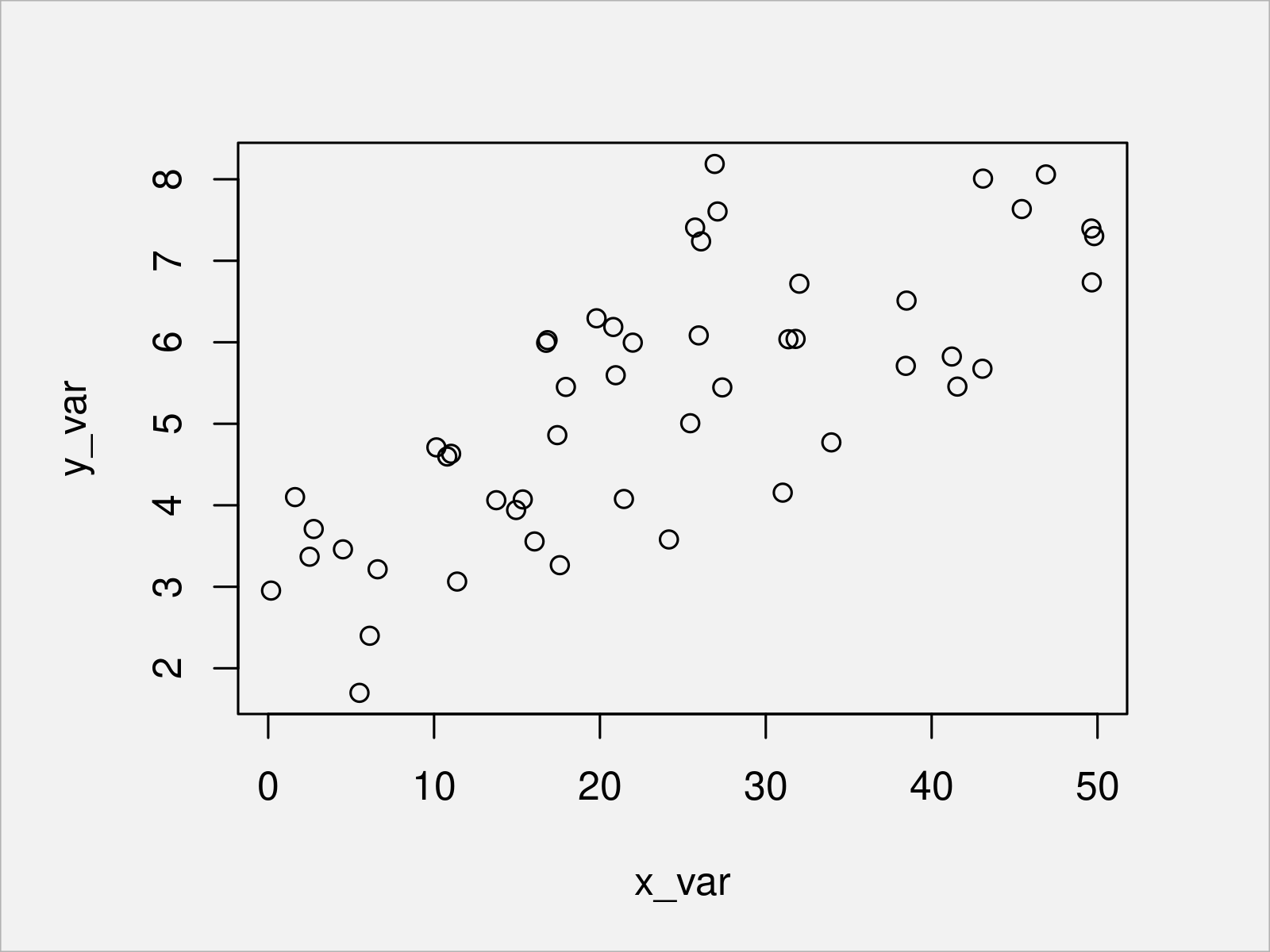
After running the previous code, the scatterplot shown in Figure 1 has been created.

Example: Generalized Cross-Validation

In this example, we apply the R code presented in the book Generalized additive models – an Introduction with R to our example data. We fit a univariate spline, as we have only one independent variable. To be more precise: We fit a penalized piecewise linear function. For the function, we have to choose a penalty parameter. We pick the parameter with generalized cross-validation (GCV). For the theory and formulas of GCV, we refer you to Chapter 4.2 of the book.

For the code, we need to define three functions, the descriptions of which are given in the Wood book, wherefore we do not repeat them in detail.

First, we define a function for the linear basis functions.

tf <- function(x, xj, j) {                            
 # Wood book page 165
 # generate jth tent function from set defined by knots xj
  dj    <- xj * 0
  dj[j] <- 1
  approx(xj, dj, x)$y
}

Next, we define a function which outputs the model matrix based on the basis functions.

tf.X <- function(x, xj) {                            
 # Wood book page 166
 # tent function basis matrix given data x
 # and knot sequence xj
  nk <- length(xj); n <- length(x)
  X <- matrix(NA, n, nk)
  for (j in 1:nk) X[, j] <- tf(x, xj, j)
  X
}

Lastly, we define a function for fitting a penalized pircewise linear smoother.

prs.fit <- function(y, x, xj, sp) {        
  # Wood book page 169
  X <- tf.X(x, xj)                                    # model matrix
  D <- diff(diag(length(xj)), differences = 2)        # sqrt penalty
  X <- rbind(X, sqrt(sp)*D)                           # augmented model matrix
  y <- c(y, rep(0,nrow(D)))                           # augmented data
  lm(y ~ X - 1)                                       # penalized least squares fit
}

For the example, we select 6 knots, equally spaced within the range of our independent variable. Using the previously defined function tf.X, we create the model matrix for the piecewise linear functions.

# Wood book page 169
sj <- seq(min(x_var), max(x_var), length = 6)         # generate knots
X  <- tf.X(x_var, sj)                                 # get model matrix
s  <- seq(min(x_var), max(x_var), length = 300)       # prediction data
Xp <- tf.X(s, sj)                                     # prediction matrix

To illustrate the behavior of the piecewise linear function under different penalty parameters, in the following, we show the resulting fits for zero penalty and two positive penalties.

sp_candidate <- c(0, 5, 10) # Three exemplary candidate values for the penalization
for (sp_i in sp_candidate) {
  b <- prs.fit(y_var, x_var, sj, sp_i)             # Re-fit
  plot(x_var, y_var, main = paste0("sp = ", sp_i)) # Plot data
  lines(s, Xp %*% coef(b), col = "red")            # Add penalized piecewise linear function
}

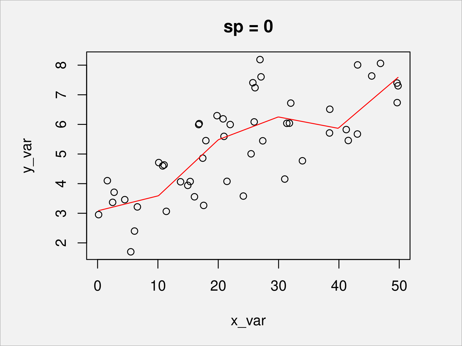
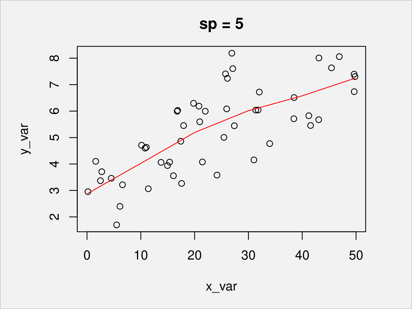
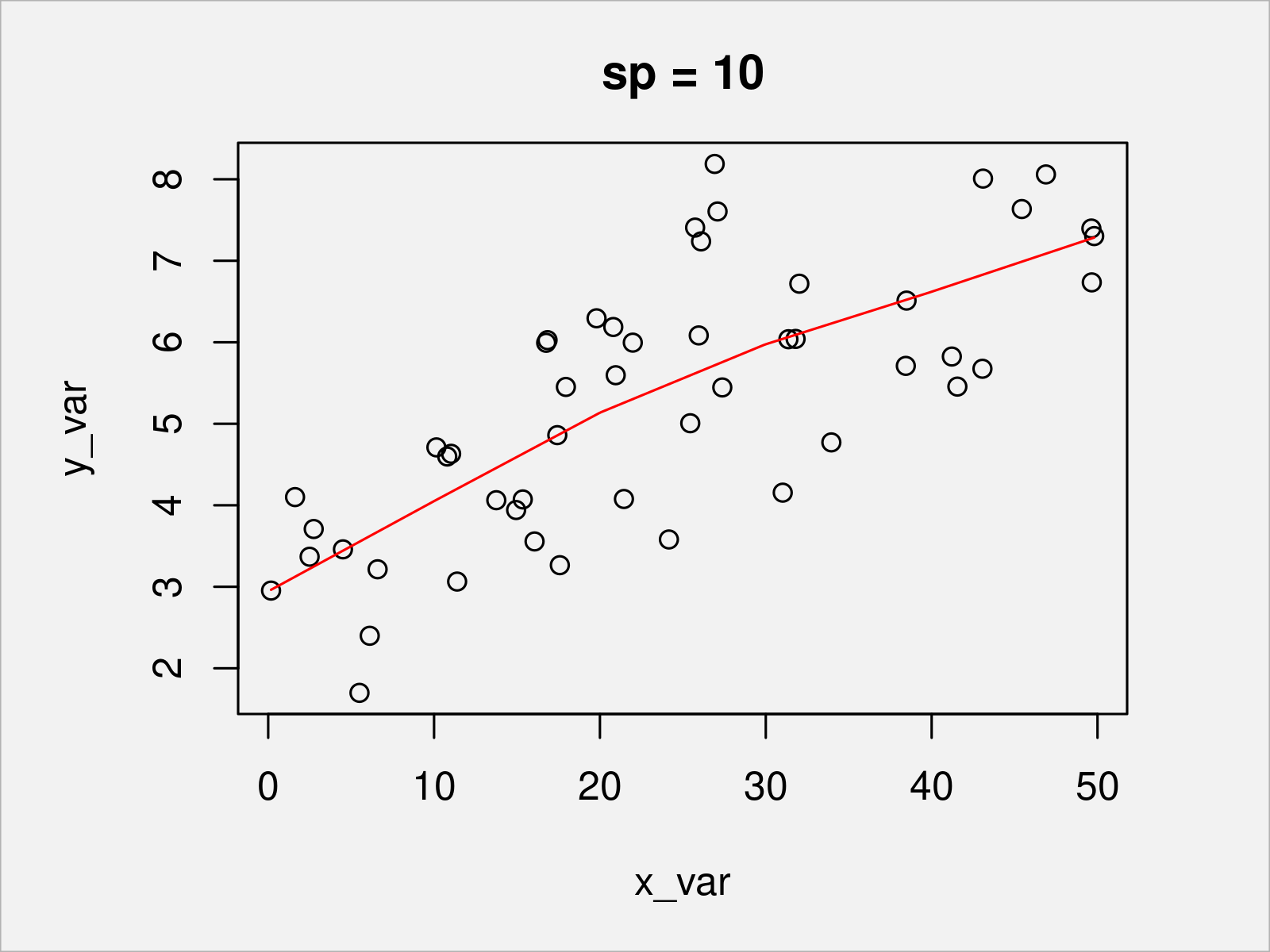
In Figures 2, 3, and 4, you can see the penalized piecewise linear function with different penalty values. The higher the penalty (which handles the curvature of the function), the smoother the resulting function.

To choose a good candidate value, that is one which generalizes well to unseen data, we can use generalized cross validation (GCV). You can see the formulas of GCV (in contrast to ordinary cross-validation) in the Wood book or this homepage of the Humboldt-Universität Berlin.

We use a grid search. That is, for each candidate value, we calculate the GCV.

# Wood book page 171-172
rho_cand <- seq(-9, 11, length = 90) # 90 candidate values, equally spread from -9 to 11
n        <- length(y_var)
V        <- rep(NA, 90)
 
for (i in 1:length(rho_cand)) {                       # loop through smoothing params
  b <- prs.fit(y_var, x_var, sj, exp(rho_cand[i]))    # fit model
  trF <- sum(influence(b)$hat[1:N])                   # extract EDF
  rss <- sum((y_var-fitted(b)[1:N])^2)                # residual SS
  V[i] <- N * rss / (N-trF)^2                         # GCV score
}

Plot the GCV score for the different candidate values.

plot(rho_cand,                                        # Plot data
     V, 
     type = "l", 
     xlab = expression(log(lambda)), 
     main = "GCV score")
sp <- exp(rho_cand[V == min(V)])                      # extract optimal sp
sp
# [1] 9.355413

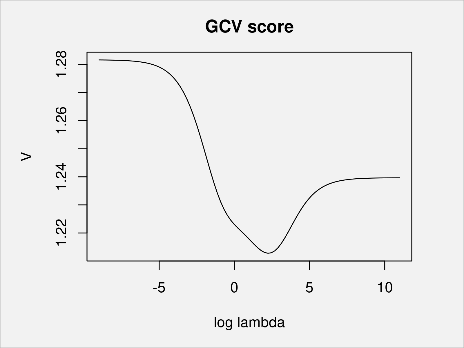
You can see that for a lambda of 9.36 (log lambda = 2.24), the GCV score is the smallest among the candidate values. We fit the penalized piecewise linear function with the chosen penalty parameter and take a look at the final fit.

b <- prs.fit(y_var, x_var, sj, sp)                    # re-fit
plot(x_var, y_var, main = paste0("GCV optimal sp = ", round(sp, 2)))
lines(s, Xp %*% coef(b), col = "red")

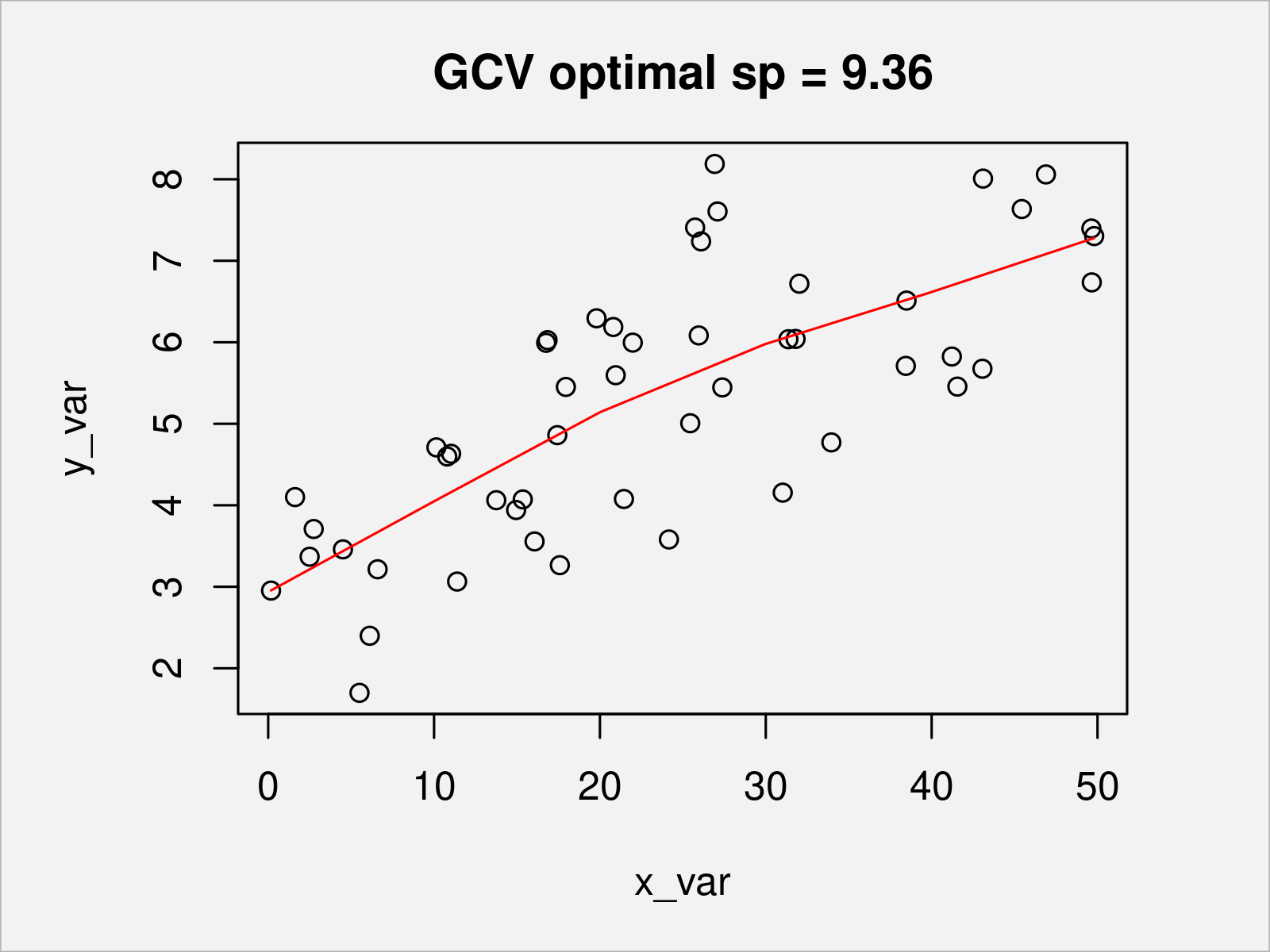
As shown in Figure 6, we have created a penalized piecewise linear function for modelling y_var via x_var. As there were only few data points, the optimal penalty parameter is rather high such that the penalized piecewise linear function is rather smooth.

Video, Further Resources & Summary

I have recently published a video tutorial on my YouTube channel, which illustrates the R code of this tutorial. Please find the video below.

The YouTube video will be added soon.

In addition, you may have a look at some related tutorials on my website. I have published several articles already.

• Stratified k-fold Cross-Validation in R (Example)
• k-fold Cross-Validation in R (Example)
• Cross-Validation Explained (Example)
• Split Data into Train & Test Sets in R (Example)
• R Programming Overview

To summarize: You have learned in this tutorial how use generalized cross validation to choose a penalty parameter for some smoothing function in the R programming language. Please let me know in the comments section, if you have any additional questions. Furthermore, please subscribe to my email newsletter to receive updates on new articles.

This page was created in collaboration with Anna-Lena Wölwer. Have a look at Anna-Lena’s author page to get further information about her academic background and the other articles she has written for Statistics Globe.