microbenchmark Package in R (2 Examples)
In this post, I’ll show how to use the microbenchmark package for comparing the performance of different algorithms in the R programming language.
The tutorial contains this information:
Let’s get started.
Example Data & Packages
First, we have to install and load the microbenchmark package to R. Furthermore, we use the ggplot2 package for visualization.
install.packages("microbenchmark")                                     # Install & load microbenchmark
library("microbenchmark")

install.packages("ggplot2")                                            # Install & load ggplot2
library("ggplot2")
Example 1: Microbenchmark Options
With the microbenchmark package, we want to compare the efficiency of different approaches for calculating the sum of the squared values of a vector. We define two different functions for that.
Function f1 uses a loop.
f1 <- function (x) {                                                   # Define function 1
  out <- 0
  for (i in 1:length(x)) {
    out <- out + x[i]^2
  }
  out
}
Function f2 uses the ability of R to directly calculate the squared values of all elements of a vector.
f2 <- function (x) {                                                   # Define function 2
  sum(x^2)
}
Now, we create a vector x with 1000 randomly drawn values from a normal distribution (using rnorm) and use the microbenchmark function to compare the performance of f1 and f2. Microbenchmark executes both functions 100 (default value) times.
set.seed(599)                                                          # Set seed for reproducible results
x <- rnorm(10000)                                                      # Generate function input
microbench_out <- microbenchmark(f1(x), f2(x))                         # Benchmark function performance
microbench_out
# Unit: microseconds
#   expr      min        lq       mean    median       uq       max neval
#  f1(x) 3534.787 3597.6230 5170.40721 3655.4045 3965.551 29759.614   100
#  f2(x)   18.733   20.4415   25.40898   26.5995   28.701    44.698   100
The output presents the summary statistics of the microseconds of the 100 executions. You can see that f2 is much faster than f1.
Let us play around with the options of the microbenchmark package. This time, we change the number of iterations from default value 100 to 1000.
microbench_out2 <- microbenchmark(f1(x), f2(x),                        # Benchmark performance with more iterations
                                  times = 1000)
microbench_out2
# Unit: microseconds
#   expr      min        lq       mean    median        uq      max neval
#  f1(x) 3527.276 3593.3040 5097.13182 3662.7825 3869.8840 35090.25  1000
#  f2(x)   17.855   19.9215   45.72353   24.8785   26.9695 21652.05  1000
Compared to the first microbenchmark output, you see that neval now takes value 1000. You can also see that the summary statistics (especially the median, lower and upper quartile) did not change much.
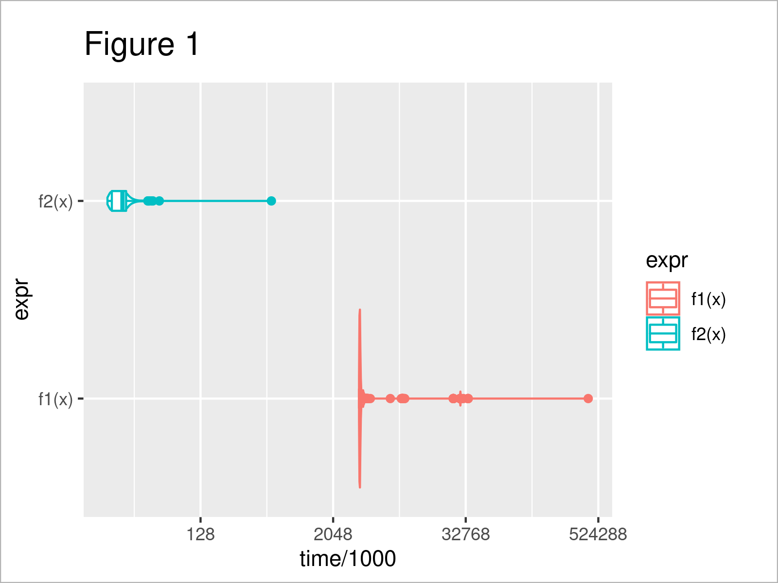
We can visualize the computation time of the 1000 iterations using ggplot.
ggplot(microbench_out2, aes(x = time/1000, y = expr, color = expr)) +  # Plot performance comparison
  geom_violin() +
  geom_boxplot(width = 0.1) +
  scale_x_continuous(trans = 'log2')

The output of the previous R syntax is shown in Figure 1 – you can see the distribution of the computation time per iteration and function.
Microbenchmark also comes with argument check. With it, you can make sure that the functions which you insert into microbenchmark actually return the same input (check = “equal”).
microbench_out3 <- microbenchmark(f1(x), f2(x),                        # Benchmark and check whether input is equal
                                  check = "equal")
microbench_out3
# Unit: microseconds
#   expr      min        lq       mean    median        uq       max neval
#  f1(x) 3529.605 3566.9810 4942.10765 3582.4990 3615.7735 29288.322   100
#  f2(x)   18.190   20.0185   24.82022   25.7995   27.5905    42.896   100
As you can see, when they return the same output, the function simply returns the typical microbenchmark output.
Now, we define x2 (which differs from x) and check again, with f1 calculated with x and f2 calculated with x2.
x2 <- x                                                                # New input x2
x2[1] <- x[1] + 1
microbenchmark(f1(x), f2(x2), # Benchmark and check whether input is equal
               check = "equal")
# Error: Input expressions are not equivalent.
As you can see, for that case, microbenchmark returns an error.
Example 2: Loop vs. Apply
In this example, we calculate the row sums of the squared values of a matrix. This time, we want to see the performance of built-in function rowSums compared to two self-written functions.
We first define two self-written functions f3 and f4. f3 uses a loop, f4 the apply function.
f3 <- function (X) {                                                   # Define function 3
  out <- vector()
  for (i in 1:nrow(X)) {
    out[i] <- sum(X[i, ]^2)
  }
  out
}
f4 <- function (X) {                                                   # Define function 4
  apply(X, 1, function (y) { sum(y^2) })
}
We create a matrix X with randomly drawn values from a normal distribution.
set.seed(963)                                                          # Set seed for reproducible results
# [1] TRUE
X <- matrix(rnorm(400, 100), nrow = 400, ncol = 100)                   # Generate input matrix
First, let us check that all three approaches return the same output using function all.equal().
all.equal(f3(X), rowSums(X^2), f4(X), tolerance = 10^(-10))            # Check whether functions return same output
# TRUE
Let us check the performance.
microbench_out4 <- microbenchmark(f3(X),                               # Benchmark performance of different functions
                                  rowSums(X^2),
                                  f4(X))

microbench_out4
# Unit: microseconds
#          expr      min        lq      mean    median        uq       max neval
#         f3(X) 1262.018 1294.3235 1778.5585 1307.0220 1320.4775 26950.455   100
#  rowSums(X^2)  126.273  134.6435  139.0888  138.7045  141.5695   165.094   100
#         f4(X) 1261.270 1284.6600 2160.9523 1296.8225 1313.6545 26949.950   100
As you see, function rowSums is – by far – the most efficient among the presented approaches.
Video & Further Resources
Some time ago, I have published a video on my YouTube channel, which demonstrates the R programming codes of this tutorial. You can find the video below.
The YouTube video will be added soon.
In addition to the video, you may read the related tutorials on this website. Some tutorials that are related to the performance comparison can be found below:
- RcppArmadillo Package in R (Example)
- Matrix Multiplication Using Rcpp Package in R (Example)
- R Programming Language
This tutorial has illustrated how to use the microbenchmark package for comparing the computational performance of different commands in R. Don’t hesitate to let me know in the comments below, in case you have further questions.
This page was created in collaboration with Anna-Lena Wölwer. Have a look at Anna-Lena’s author page to get further instructions about her academic background and the other articles she has written for Statistics Globe.


