Extract eCDF Values from ecdf Function in R (Example)

In this tutorial, I’ll explain how to extract the eCDF values from the ecdf() function in R programming.

The page contains these contents:

Let’s get started.

Creation of Example Data

The first step is to create some example data:

set.seed(456383)                       # Set seed for reproducibility
x <- rnorm(100)                        # Generate random values from normal distribution
head(x)                                # Print first six values
# [1] -1.8431654399  0.8026014150 -1.1282631488  1.1752683833 -0.8225131337 -0.0698087629

The previous output of the RStudio console illustrates that our exemplifying data is a vector containing 100 normally distributed random values.

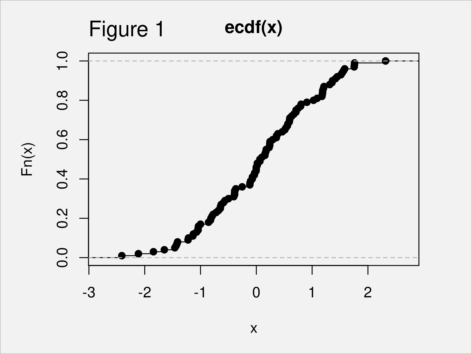
Now, we might plot the data in an empirical Cumulative Distribution graph using the ecdf function as shown below:

plot(ecdf(x))                          # Create ecdf plot in R

Figure 1 shows the output of the previous R code: We have drawn an eCDF plot.

However, let’s assume that we want to extract the values from this eCDF graphic…

Example: Extract eCDF Values from ecdf() Function

The R code below shows how to return the eCDF values when using the ecdf() function in R.

First, let’s apply the ecdf() function to our example data, and let’s store the output in a new object called fun_ecdf:

fun_ecdf <- ecdf(x)                    # Create ecdf function

The fun_ecdf object is actually a function. You can see that by applying the class command to fun_ecdf:

class(fun_ecdf)                        # Check class
# [1] "ecdf"     "stepfun"  "function"

We may now use this function to return the eCDF values corresponding to our example data:

my_ecdf <- fun_ecdf(x)                 # Apply ecdf function
my_ecdf                                # Print output of function
#   [1] 0.03 0.78 0.12 0.82 0.19 0.41 0.64 0.60 0.90 0.34 0.10 0.57 0.50 0.43 0.02
#  [16] 0.06 0.86 0.18 1.00 0.67 0.97 0.35 0.94 0.46 0.74 0.79 0.71 0.72 0.05 0.63
#  [31] 0.08 0.56 0.21 0.53 0.77 0.11 0.55 0.27 0.96 0.66 0.61 0.75 0.16 0.91 0.81
#  [46] 0.31 0.88 0.14 0.89 0.01 0.17 0.04 0.47 0.83 0.73 0.87 0.25 0.24 0.45 0.20
#  [61] 0.51 0.65 0.33 0.69 0.38 0.32 0.30 0.07 0.28 0.42 0.84 0.98 0.62 0.13 0.23
#  [76] 0.99 0.09 0.39 0.49 0.40 0.68 0.52 0.76 0.48 0.92 0.70 0.59 0.37 0.26 0.22
#  [91] 0.44 0.58 0.29 0.36 0.54 0.85 0.95 0.93 0.15 0.80

Looks good.

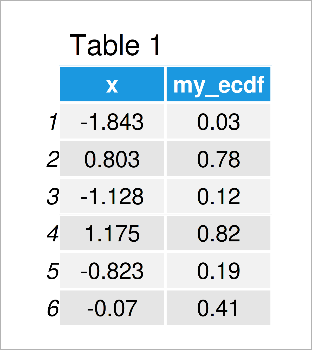
We might also combine these eCDF values with our input data in a data.frame object.

Consider the R syntax and its output below:

data_ecdf <- data.frame(x, my_ecdf)    # Combine x & eCDF values
head(data_ecdf)                        # Print head of data frame

Note that we could also create a list, matrix, tibble, or whatever we want based on these data.

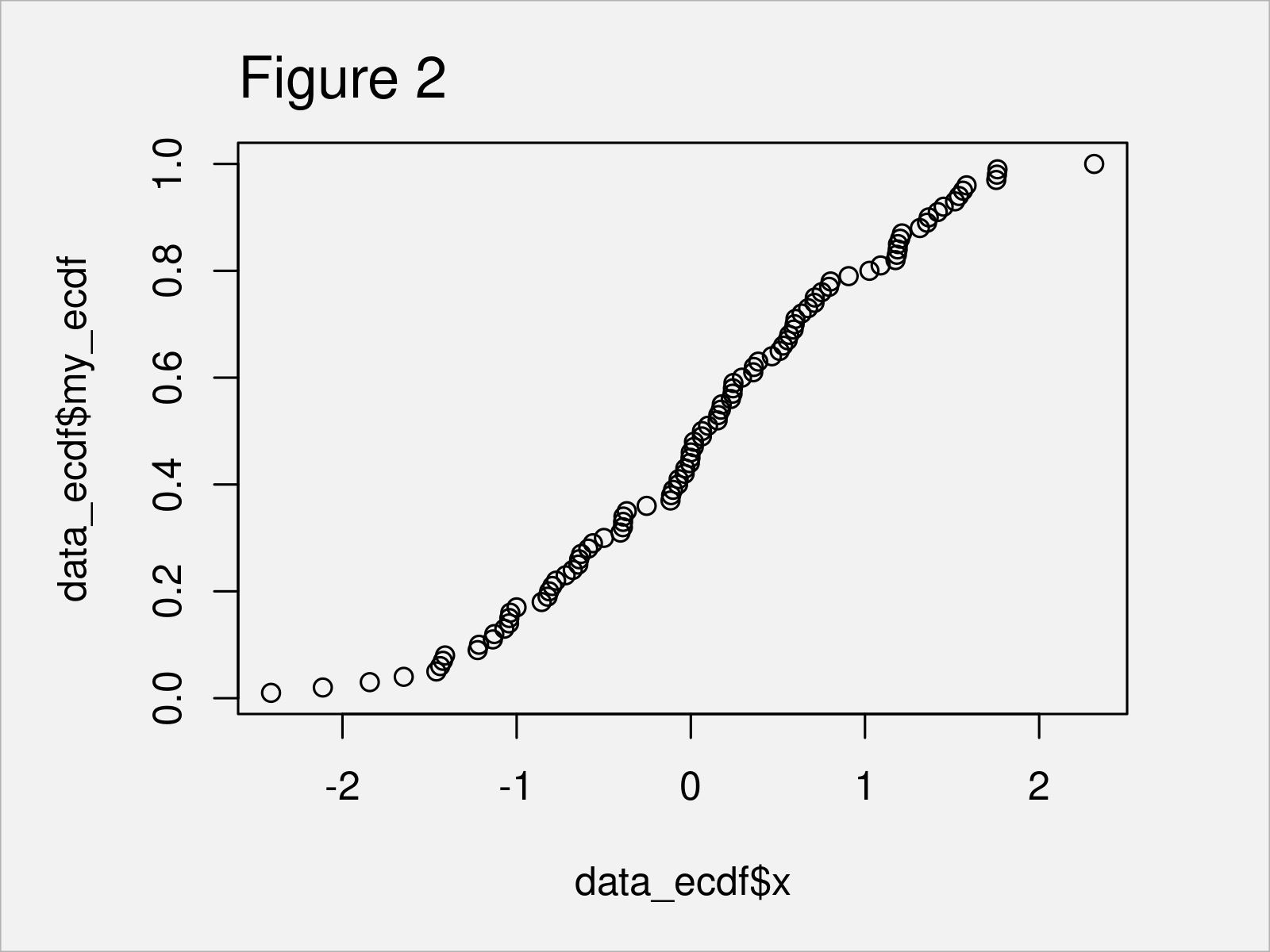
We may now use the plot function to draw our eCDF plot once again based on our data frame:

plot(data_ecdf$x,                      # Plot eCDF values once again
     data_ecdf$my_ecdf)

By executing the previous R code, we have created Figure 2. As you can see, the style of the plot is slightly different compared when plotting the output of the ecdf() function. However, the displayed data points are exactly the same.

Video & Further Resources

In case you need further explanations on the content of this tutorial, I recommend watching the following video on my YouTube channel. In the video, I’m explaining the content of this article in RStudio.

Furthermore, you may want to have a look at some of the other tutorials on my website:

• Extract Values from Matrix by Column & Row Names
• Extract Values & Names from table Object
• Extract Fitted Values from Regression Model in R
• Extract Unique Values in R
• Important Commands in R
• All R Programming Tutorials

To summarize: In this article, I have shown how to get and return eCDF data from the ecdf() function in the R programming language. If you have further questions and/or comments, let me know in the comments below.