What is Explainable AI? | Principles, Benefits & Example Code in Python

This page contains a guest article provided by Ines Röder. Ines is a survey statistician and data scientist at the targens GmbH. You may find more information about Ines on her Statistics Globe profile page.

“I don’t trust complex models because they are black-boxes.” You may have heard in the past. But what are black-boxes and what is explainability?

Let’s start from the beginning. Let’s assume that our friend Tim approaches us with the following problem: He wants to build a model to predict the income. Tim uses a linear model for this purpose.

\(\hat{f}(X_i) = \hat{Y}_i = \hat{\beta}_0 + \hat{\beta}_1 X_i + \hat{\epsilon}_i\)

A linear model is very well explainable and comprehensible. The influence of a single model variable on the model prediction is clearly visible. Other examples of simple and explainable models are decision trees, logistic regressions or decision rules.

So why not always use a interpretable model?

If the relationship of the variables isn’t linear or the problem is more complex, the performance of simple and interpretable models can be very poor. More complex models like random forests or neural nets have to be considered. They have the problem that they are not well explainable.

These complex models are also called black boxes. The input data is given to the model, which delivers a prediction, e.g. 2,000€ for the income of person-1. However, it is not clear how the model arrives to this prediction. Hence, they are named black box models. Especially for real-world problems, it is important that the models are explainable. For example, when models are used for medical prognosis or in the highly regulated financial markets. However, simple explainable models are often not sufficient for these complex problems.

Tim asks himself: What to do now? Should I choose an explainable model which has a poor performance for my problem or a complex model which is not explainable?

Fortunately in the last years, there has been a growth of explainability methods. These methods make it possible to explain black box models. Here, a distinction has to be made between global and local explainability:

• Global explainability provides inferences for the entire model. Over all observations, how important was the variable “work experience” (in years)?
• Local explainability, on the other hand, considers the explanation for a single observation. For example: Why was the income of person-1 estimated at 2,000€? The amount of influence of the variable “work experience” for this specific prediction is calculated.

In this article, we focus on the explainability methodology SHAP (Shapley Additive exPlanations). For a detailed overview of explainability methods, the book by Christopher Molnar (Interpretable Machine Learning) is recommended.

SHAP (Shapley Additive exPlanations)

SHAP is based on game theory. Example: we have a game with three players (A, B, C). At the end, there is a win. This should be distributed fairly to the players. The player who has contributed the most gets the most.

Example: If player A plays alone he gets 25 €, player B 50€ and player C 100€. players A and B together receive 300 €, A and C 400 € and B and C 600€. All players together receive 900€.

Table 1: Game Theory Example

The marginal contributions of the combination ABC has to be calculated.

Therefore, all different sequences are considered, e.g.

• If player A is the first one he gets 25€
• If player B is the second player he gets 275€ : 300€ (AB together) – 25€ (for player A)
• Player C gets 600: 900€ (ABC together) – 300€ (AB)

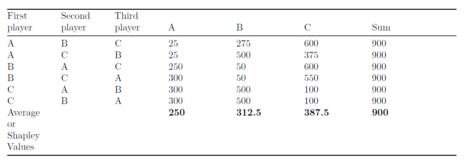
Table 2: Example Shapley Values

The Shapley Values, the marginal contributions, are the average win for each player over all possible combinations.

SHAP is based on the idea of the game theory. Instead of players, there are variables which have a contribution to the model prediction (the “profit”). We are interested in how much each variable has contributed to the model prediction. So, all different variable coalitions are considered and the marginal contributions are calculated.

The goal of SHAP is to explain the difference between an average model prediction and the prediction for a specific observation.

For example, for the linear model is the contribution \(\alpha\) for the feature \(j\) :

\(\alpha_{j} = \beta_{j} X_{j} – E(\beta_{j} X_{j}) ,\)

where \(E(\beta_{j} X_{j})\) is an estimate of the mean effect. This is calculated for each feature and every prediction. The example is only for a linear model. Shapley Values can be calculated for any model. For a detailed statistical explanation of Shapley Value see here.

Depending on the chosen model, different SHAP calculations are possible, e.g. TreeSHAP for tree-based models. Each method has its advantages and disadvantages, of course. KernelSHAP is for every model possible but has a lot of computational costs.

In the following Python example, we will focus on TreeSHAP. For a simple and well understandable explanation for TreeSHAP, this article is recommended.

Python Example

import shap
import pandas as pd
import sklearn
from sklearn.ensemble import RandomForestClassifier
from sklearn.datasets import make_classification
from sklearn.preprocessing import OneHotEncoder
import numpy as np

Before we can continue with the Python syntax, we first have to download the example data that we’ll use in this example. You can find the data here.

Once the data is downloaded, you can import it to Python by specifying your directory path as demonstrated below:

# Explainability with SHAP
## Shapley Additive Explanations
 
## load the data
df = pd.read_csv('../Downloads/electricity_zip/data/electricity_csv.csv') ## your path

Information about the features

Independent variables:

• date: 7 May 1996 to 5 December 1998, normalized between 0 and 1
• day: weekday from 0 to 7
• period: Units for measuring time (1-48), normalized between 0 and 1
• nswprice: New South Wales electricity price, normalized between 0 and 1
• nswdemand: New South Wales electricity demand, normalized between 0 and 1
• vicprice: Victoria electricity price, normalized between 0 and 1
• vicdemand: Victoria electricity demand, normalized between 0 and 1
• transfer: planed electricity transfer between Victoria and New South Wales, normalized between 0 and 1

Dependent variable:

• class: change of the price (up or down) for New South Wales for the last 24 hours

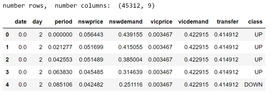
print('number rows, ', 'number columns: ', df.shape)
 
df.head() ## short look at the dataframe

X_names = list(df.columns)
X_names.remove('class')    ## delete class - only the independent variables are left
 
y_names = 'class'          ## dependent variable
print(X_names, y_names)

## Some statistics
#missing value - check
#summary statistics
#note: a detailed analysis of the data is not provided here
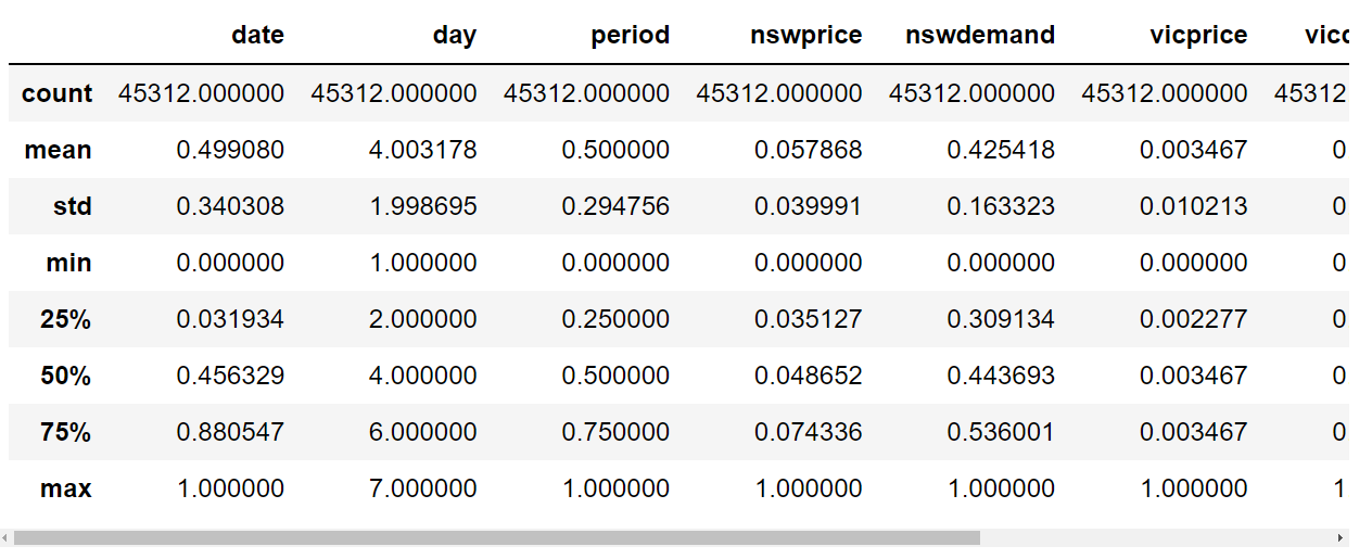
print(df.isna().sum()) ## no missing values
print(df.describe())

### Train the model
# A random forest - documentation to the model:
# https://scikit-learn.org/stable/modules/generated/sklearn.ensemble.RandomForestClassifier.html
 
from sklearn.model_selection import train_test_split
from sklearn.preprocessing import LabelEncoder
 
label_enc = LabelEncoder()
df[[y_names]] = pd.DataFrame(label_enc.fit_transform(df[[y_names]])) ## encode the class variable
 
train, test = train_test_split(df, test_size=0.3, random_state = 4) ## split the data to a test and train dataframe
print(len(train), len(test))

train.head()

from sklearn.metrics import confusion_matrix
from sklearn.metrics import precision_score, recall_score, f1_score, accuracy_score
import matplotlib.pyplot as plt
 
clf = RandomForestClassifier(max_depth=2, n_estimators=50, random_state=0)
clf.fit(train[X_names], np.ravel(train[[y_names]])) ## fit the model
 
conf_matrix_train = confusion_matrix(y_true=np.ravel(train[[y_names]]), y_pred=clf.predict(train[X_names]))
 
fig, ax = plt.subplots(figsize=(5, 5))
ax.matshow(conf_matrix_train, cmap=plt.cm.Greens, alpha=0.6)
 
for i in range(conf_matrix_train.shape[0]):
    for j in range(conf_matrix_train.shape[1]):
        ax.text(x=j, y=i,s=conf_matrix_train[i, j], va='center', ha='center', size='xx-large')
 
plt.xlabel('Predictions', fontsize=12)
plt.ylabel('Actuals', fontsize=12)
plt.title('Confusion Matrix - Train', fontsize=12)
plt.show()
 
conf_matrix_test = confusion_matrix(y_true=np.ravel(test[[y_names]]), y_pred=clf.predict(test[X_names]))
fig, ax = plt.subplots(figsize=(5, 5))
ax.matshow(conf_matrix_test, cmap=plt.cm.Greens, alpha=0.6)
 
for i in range(conf_matrix_test.shape[0]):
    for j in range(conf_matrix_test.shape[1]):
        ax.text(x=j, y=i,s=conf_matrix_test[i, j], va='center', ha='center', size='xx-large')
 
plt.xlabel('Predictions', fontsize=12)
plt.ylabel('Actuals', fontsize=12)
plt.title('Confusion Matrix - Test', fontsize=12)
plt.show()
 
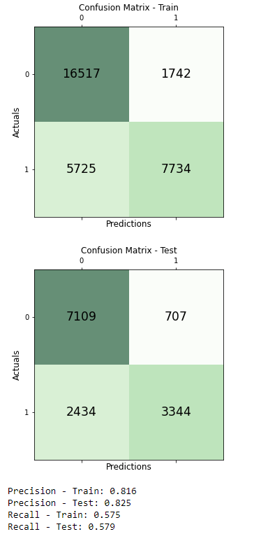
print('Precision - Train: %.3f' % precision_score(train[[y_names]], clf.predict(train[X_names])))
print('Precision - Test: %.3f' % precision_score(test[[y_names]], clf.predict(test[X_names])))
print('Recall - Train: %.3f' % recall_score(train[[y_names]], clf.predict(train[X_names])))
print('Recall - Test: %.3f' % recall_score(test[[y_names]], clf.predict(test[X_names])))
 
 
### The model is not optimal and has to be optimized
### For further optimizing of the model see:
### https://nyandwi.com/machine_learning_complete/20_random_forests_for_classification/#7-improving-random-forests

import shap
 
explainer = shap.TreeExplainer(clf)
shap_values = shap.TreeExplainer(clf).shap_values(train[df[X_names].columns])
shap.summary_plot(shap_values[1], train[X_names], plot_type="bar") ## global explanation

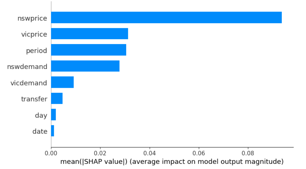
The most important feature is nswprice, it has the highest mean absolute SHAP-value. This is the average influence of the feature over all training data.

shap.summary_plot(shap_values[1], train[X_names], plot_type = 'dot') ## global explanation
 
# colors: red - the value of the feature is high
#         blue - the value of the feature is low

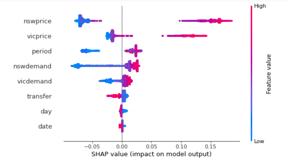
Every point is the SHAP-value for one observation and one feature. The SHAP values over the training data are shown. Every feature with a negative SHAP-value reduce the probability for an increasing price. Features with a positive SHAP-value increase the probability for an increasing price.

• The probability for an increasing price will be reduced for a low nswprice, period, …
• The probability for an increasing price will be increased for a high vicprice, vicdemand, nswdemand, …

## local Explainability
# load JS visualization code to notebook
shap.initjs()
# visualize the sixth prediction’s explanation
shap.force_plot(explainer.expected_value[1], shap_values[1][5,:], train[X_names].iloc[5,:])

The base value is 0.4239. It is the mean probability in the training data for a change in the price to rise. The probability for the chosen observation is 0.38 for a change in price to rise. In reverse is the probability for the chosen observation 0.62 for a change in price to reduce. So the probabilities sum up to one. The SHAP values describes the difference from the base value to the actual prediction. If we add all the SHAP values to the base value we would get the model output (here 0.38).

base_value = explainer.expected_value[1]
pred_2 = base_value + np.sum(shap_values[1][2,:])
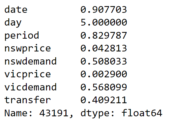
print(shap_values[1][2,:]) ## SHAP values
print(base_value, pred_2)  ## base value and prediction

For this local observation are the \(nswprice\) and the \(vicprice\) the main reasons that the model predicts the price to be increased.

train[X_names].iloc[2,:] ## feature values of observation 2

Explainable artificial intelligence and machine learning are growing areas of research, and it is exciting to see how it will continue to develop. It is therefore worthwhile to look for the benefits of new methodologies or extensions of existing principles and methodologies.