Calculate Leverage Statistics in R (Example)

In statistics, being able to identify extreme x values is a key to understand our analysis: in some situations, these extreme values may influence our regression model.

Similar to an outlier, which is defined as an observation that lies in abnormal distance from other values in a sample, leverage measures how far away the data point is from the mean value. Thus, leverage statistics help us to identify extreme x values.

In order to be able to measure the impact on the results of our model, we can calculate the leverage in our observations.

In this article you’ll learn how to calculate leverage statistics for each observation in a model in the R programming language.

The table of content has the following structure:

Let’s dive into it.

Creation of Example Data and Regression Model

For this tutorial, we will use the following data:

set.seed(999)
x1 <- rnorm(10)
x2 <- rnorm(10) + 0.15 * x1
x3 <- rnorm(10) + 0.30 * x1
y <- rnorm(10) + 0.1 * x1 + 0.35 * x2 - 0.2 * x3
example_data <- data.frame(x1,x2,x3,y)
example_data

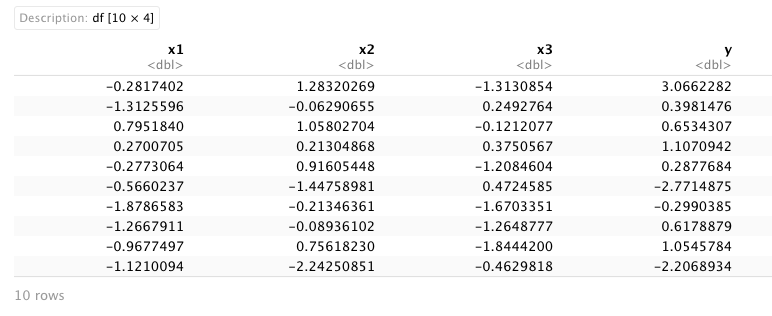
As you can see on the RStudio output, our example data contains four numeric columns: the variables x1-x3 as predictors and the variable y as target variable. Now, using this data, we will build a multiple linear regression model.

Based on our data, we can estimate a linear regression model by using the lm() function:

# Fit our regression model
model_1 <- lm(y ~ ., example_data)
 
# Print summary statistics of our model
summary(model_1)

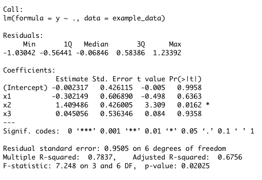
Once we have our model constructed, we can now calculate the leverage for each observation in our linear model.

Calculate the Leverage Statistics Using the hatvalues() Function

In order to calculate the leverage statistics for our regression model, we can use the hatvalues() function:

# Get leverage for each observation in the data set
leverage <- as.data.frame(hatvalues(model_1))
 
# Print leverage for each observation
leverage

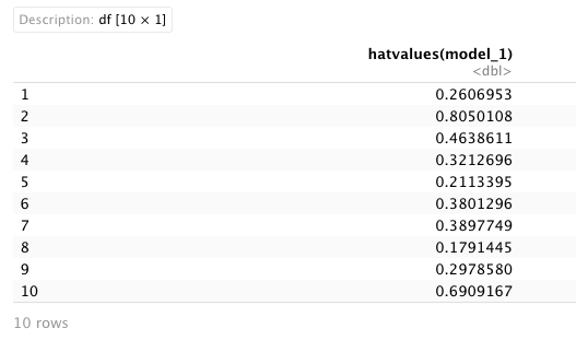
We have calculated the leverage statistics for every observation in our linear regression model. But typically, we may take a look at observations that have a higher value.

In order to achieve this, we can order all the observations from the greatest to the lowest value:

leverage[order(-leverage['hatvalues(model_1)']), ]
# [1] 0.8050108 0.6909167 0.4638611 0.3897749 0.3801296 0.3212696
# [7] 0.2978580 0.2606953 0.2113395 0.1791445

As we can see, the largest leverage value is 0.8050.

We can also plot our leverage statistics so that we can visualize the leverage for each point:

barplot(hatvalues(model_1), 
        col = "aquamarine3")

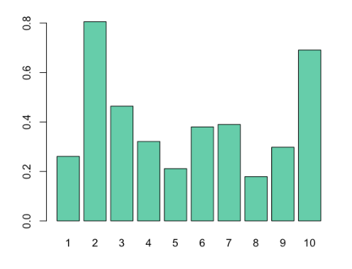
The x-axis shows the index of each point in our data frame, and the y-value shows the leverage statistics for each point.

Video, Further Resources & Summary

Do you need more explanations on how to calculate leverage statistics in R? Then you should have a look at the following YouTube video of the Statistics Globe YouTube channel.

The YouTube video will be added soon.

Furthermore, you could have a look at some of the other tutorials on Statistics Globe:

• Calculate Multiple Summary Statistics by Group in One Call
• Calculate a Binomial Confidence Interval in R
• Summary Statistics for data.table in R

This post shows how to compute leverage statistics in R. In case you have further questions, you may leave a comment below.

This page was created in collaboration with Paula Villasante Soriano. Please have a look at Paula’s author page to get more information about her academic background and the other articles she has written for Statistics Globe.