Battese-Harter-Fuller Small Area Estimator (R Example) | Unit-Level Model
We show you the Battese-Harter-Fuller (BHF) model, the most famous unit-level Small Area Estimation (SAE) model. To do this, we first review the theory of the model. Building on the theory, we create sample data and compute the model on that data in the R programming language.
The post is divided into the following blocks:
So let’s go straight to the Battese-Harter Fuller model!
Theory of the Battese-Harter-Fuller Model
If you are new to the topics of survey estimation and small area estimation, check out our article about small area estimation first. We use model-based small area models to improve survey estimates, especially for small areas, by using auxiliary information.
The Battese-Harter-Fuller Model is probably the best known unit-level small area model. The model is named after the article by Battese, Harter, and Fuller (1988). We can use it when we have both the auxiliary information and the survey information at the unit level. In a household survey, such as the American Community Survey (ACS), the households, or the people in the households, are the units of the survey.
Consider a population \(U\). As an example, one could consider all households in the U.S. and be interested in measuring the average household consumption of a product in the U.S. counties of a specific state. In small area terms, the \(D\) counties in the state are our domains of interest, the average household consumptions per county are our parameters of interest which we denote by \(\mu_d\), \(d=1,\ldots,D\).
We can conduct a survey to estimate various county- and state specific household parameters such as \({{\mu}}_d\). Depending on the total sample size and design of the survey, it can happen that the survey direct estimates \(\hat{{\mu}}_d^{Dir}\) are precise enough for the estimation of state, but not county parameters.
In addition to the survey direct estimates, we can calculate predictions of \({{\mu}}_d\) based on the BHF model. The BHF model is given by
\begin{equation}
{y}_{di} = \boldsymbol{x}_{di}^{\top} \boldsymbol{\beta} + u_d + e_{di},\quad i=1,\ldots,N_d,\quad d=1,\ldots,D.
\end{equation}
We go through each component of the formula.
- \(N_d\) is the size of domain \(d\), for example the number of households in a specific county. The population in domain \(d\) is denoted by \(U_d\).
- \(y_{di}\) is the value of a variable of interest \(Y\) for unit \(i\) in domain \(d\). For example, the expenditure of a household \(i\) for a specific good.
- \(\boldsymbol{x}_{di}\) is a \(p\)-vector of auxiliary information for unit \(i\) in domain \(d\) which we use for the model. For example, the income, age distribution, and number of persons of the household.
- \(\boldsymbol{\beta}\) is a vector of \(p\) fixed effects associated with the auxiliary information. Note that in the model we assume that the relationship of the auxiliary information an \(\boldsymbol{\beta}\) is the same for all \(N\) units.
- \(u_d\), with \({u}_{d}\overset{iid}{\sim}N(0,\sigma^2_{v})\), is a domain-specific random effect.
- \(e_{di}\), with \({e}_{di}\overset{iid}{\sim}N(0,\sigma^2_{e})\), is a household-and-domain-specific residual.
- We assume that the random effects and residuals are independent.
From the model, we can see why the BHF model is called nested error regression (NER) model. The units \(i\) are nested within non-overlapping domains \(d\). All units of a domain \(d\) are exposed to the same realization of the domain-specific random effect \(u_d\).
The variance components \(\sigma^2_{v}\) and \(\sigma^2_{e}\) and the fixed effects vector \(\boldsymbol{\beta}\) are typically unknown and can be estimates using Maximum Likelihood (ML) or Restricted Maximum Likelihood (REML). For that, the assumptions about the distribution of the \(u_d\) and \(e_{di}\) are crucial. The estimates are denoted by \(\hat{\sigma}^2_{v}\), \(\hat{\sigma}^2_{e}\), and \(\hat{\boldsymbol{\beta}}\).
We can then apply linear mixed model (LMM) theory, to calculate the Empirical Best Linear Unbiased Predictions (EBLUPs) under the BHF model for any function of the \(y_{di}\). In the easiest case, we are interested in estimating a linear function in \(y_{di}\), like the domain means
\begin{equation}
\mu_d = \frac{1}{N_d} \sum_{i=1}^{N_d} y_{di},\quad i=1,\ldots,N_d,\quad d=1,\ldots,D.
\end{equation}
From the survey, with \(s_d\) and \(n_d\) we denote the sample and sample size in domain \(d\). We further need auxiliary information on \(\bar{\boldsymbol{x}}_{U_d}=\frac{1}{N_d} \sum_{i\in U_d} \boldsymbol{x}_{di}\), the population means of the \(p\) auxiliary variables in each domain \(d\).
The BHF EBLUPs of \(\mu_d\) are given by
\begin{equation}
\hat{\mu}_d^{EBLUP} = \bar{\boldsymbol{x}}_{U_d}^{\top} \hat{\boldsymbol{\beta}} + \hat{\gamma}_d (\bar{y}_d – \bar{\boldsymbol{x}}_d \hat{\boldsymbol{\beta}}),\quad d=1,\ldots,D,
\end{equation}
with shrinkage factor
\begin{equation}
\hat{\gamma}_d = \frac{\sigma^2_u}{\sigma^2_u + \sigma^2_e / n_d},\quad d=1,\ldots,D
\end{equation}
and sample means
\begin{equation}
\bar{y}_d = \frac{1}{n_d} \sum_{i\in s_d} y_{di}, \quad \bar{\boldsymbol{x}}_d = \frac{1}{n_d} \sum_{i \in s_d} \boldsymbol{x_{di}}.
\end{equation}
With the mixed model theory, we can also derive MSE estimators of the BHF EBLUPs. For more information on LMMs, take a look at the books Mixed Models and A Course on Small Area Estimation and Mixed Models.
In applications of BHF models, the main difficulty (besides data acquisition) is to select the auxiliary information, specify the BHF model, and evaluate the model choice given the data.
Please note that here we only take a look at the estimation of domain averages of \(y_{di}\). For non-linear functions in \(y_{di}\), the model gets more complicated. Take a look at the R Journal article for the sae package, Example 5: Poverty mapping, for an example.
Creating Example Battese-Harter-Fuller Data
We cannot only use the BHF model to model data, but also to generate data from the model. For that, we have to choose all the model parameters.
We choose a population of size \(N=200000\) (for example persons or households) and \(D=30\) domains of interest (for example specific counties). Furthermore, we set a seed to make our results, which depend on random variables, reproducible.
D <- 30       # Number of domains
N <- 200000   # Number of units in the population
set.seed(621) # Seed for reproducible results
We randomly assign each population unit to one of the 30 domains.
d_member <- factor(sort(sample(x       = 1:D,
                               size    = N,
                               replace = TRUE)),
                   labels = paste0("d", 1:D))
N_d <- table(d_member) # Domain sizes
range(N_d) # The range of the domain sizes
# [1] 6548 6833
For the fixed effects vector \(\boldsymbol{\beta}\), the residual variance \(\sigma^2_{e}\) and the variance of the random effects \(\sigma^2_{u}\), we set the following values.
beta     <- c(1, 2, 3)
sigma2_e <- 2
sigma2_u <- 2
We selected three fixed effects in \(\boldsymbol{\beta}\). The first is for a model intercept, the last two are for additional auxiliary variables. For the two variables, we randomly draw uniform numbers between 10 and 20. Also, we create the matrix of auxiliary information with and without the intercept in objects x and x_with_int.
x           <- sapply(1:2, function (i) { runif (n = N, min = 10, max = 20) })
x_with_intc <- cbind(1, x) # Auxiliary matrix with intercept as first column
We have all the parameters which we need for the model. From the residual and random effect distribution, random numbers can be drawn.
e_di       <- rnorm(N, mean = 0, sd = sqrt(sigma2_e))  # Draw residuals
u_d        <- rnorm(D, mean = 0, sd = sqrt(sigma2_u))  # Draw random effects
names(u_d) <- paste0("d", 1:D)
To rightfully assign the random effects to the domains in the data, create a dataset dat_U containing all unit-level information on the population \(U\).
if (!require('data.table', quietly = TRUE)) { install.packages('data.table') }
library('data.table') # Load package 'data.table'

dat_U <- data.table("d_member" = factor(d_member, levels = paste0("d", 1:D)),
                    "x"        = x_with_intc)
# d_member: Domain membership indicator
# x:        Auxiliary information

dat_U[, x.beta := x_with_intc %*% beta]
dat_U[, y_di   := dat_U$x.beta + u_d[dat_U$d_member] + e_di] # Population values of Y
The created variable \(y_{di}\) is our dependent variable in the BHF model.
Now, we conduct a survey. For illustration, we apply simple random sampling without replacement and draw a 0.5% sample from the population.
n = N / 200 # Sample size
sample_units <- sort(sample(x       = 1:N,
                            size    = n,
                            replace = FALSE))
n_d <- dat_U[sample_units, table(d_member)] # Domain specific sample sizes
With the generated data, we can calculate a BHF model.
Calculating the Battese-Harter-Fuller Model
There are already functions for the BHF model in the R package sae.
if (!require('sae', quietly = TRUE)) { install.packages('sae') }
library('sae') # Load package 'sae'
We use function pbmseBHF to calculate the BHF model. You can find its documentation here.
?pbmseBHFFor the BHF model, we define the population means of the auxiliary variables and the domain sizes as objects meanxpop and popnsize. Attention! In our example, the domain memberships and variables are nicely ordered. In praxis, you have to be really careful that you include domain identifiers in case some objects have a different ordering.
meanxpop                <- dat_U[, list(mean(x.V2), mean(x.V3)), by = d_member]
colnames(meanxpop)[2:3] <- c("x.V2", "x.V3")
popnsize                <- data.table(N_d)
colnames(popnsize)[2]   <- "N_d"

mod_BHF <- pbmseBHF(formula  = y_di ~ x.V2 + x.V3,
                    dom      = d_member,
                    meanxpop = meanxpop,
                    popnsize = popnsize,
                    method   = "REML",
                    data     = dat_U[sample_units, ],
                    B        = 50)
# formula:  y_di is the dependent variable,
#           x.V2 and x.V3 are the auxiliary variables.
#           The model automatically considers an intercept.
# dom:      Domain identifier.
# meanxpop: County means of x.V2 and x.V3.
# popnsize: Domain sizes N_d.
# method:   Method used for estimating the model parameters,
#           REML is restricted maximum likelihood.
# B:        Number of bootstrap replicates. Default is 50.
That’s it. We just calculated a BHF model. As we know the true fixed effects and variances which we used to generate the data, we can take a look at whether our estimates are close.
# Fixed effects
beta                     # True
# [1] 1 2 3
mod_BHF$est$fit$fixed    # Estimated
# XsXs(Intercept)        XsXsx.V2        XsXsx.V3
#       0.4641307       2.0209279       3.0175522

# Variance of domain random effects
sigma2_u                 # True
# [1] 2
mod_BHF$est$fit$refvar   # Estimated
# [1] 2.312924

# Variance of residuals
sigma2_e                 # True
# [1] 2
mod_BHF$est$fit$errorvar # Estimated
# [1] 1.765405
We can see that the estimates values are close. You can vary the parameters like the number of domains, the seed, and the population size to see how the estimates change. When you conduct a Monte Carlo simulation study using the data generation and estimation with varying seed, you can see whether the parameter estimation is unbiased. Have a try!
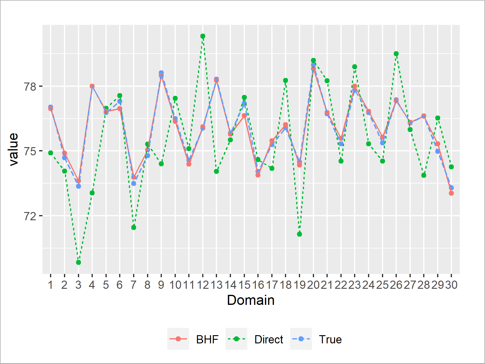
From object mod_BHF, we get the model EBLUPs and MSEs via mod_BHF$est$eblup and mod_BHF$mse. We can start by visually taking a look at the resulting estimates compared to the true values.
  if (!require('ggplot2', quietly = TRUE)) { install.packages('ggplot2') }
library('ggplot2') # Load package 'ggplot2'

mu_dir   <- dat_U[sample_units, mean(y_di), by = d_member]$V1 # Direct estimates from the survey
BHF_est  <- mod_BHF$est$eblup$eblup                           # BHF EBLUPs
mu       <- dat_U[, mean(y_di), by = d_member]$V1             # True domain averages

# Put all information in one data.table object
dat_plot <- data.table("Estimator" = c(rep("True", D), rep("Direct", D), rep("BHF", D)),
                       "Domain"    = factor(c(1:D, 1:D, 1:D)))
dat_plot[, value := c(mu, mu_dir, BHF_est)]

# Plot the data
ggplot(data = dat_plot,
       aes(x     = Domain,
           y     = value,
           group = Estimator,
           lty   = Estimator,
           color = Estimator)) +
  geom_point(pch = 19) +
  geom_line() +
  theme(legend.position = "bottom",
        legend.title = element_blank()) +
  scale_y_continuous("value")

We see that the BHF EBLUPs are pretty close to the true domain averages. Nice! The direct estimates, on the other hand, have much more variation around the true values.
As a task for yourself: Find the right variance formula for the direct domain estimates under simple random sampling without replacement and compare the coefficient of variation of the BHF EBLUPs and direct estimates! As a hint, you can find the formulas in the book Model-Assisted Survey Sampling.
Video, Further Resources & Summary
In our article about Small Area Estimation in R, we also provide a concrete example of the BHF model.
You want to learn more about the BHF model? We recommend you to have a look at the book Small Area Estimation. One of the authors, Isabel Molina, is also one of the authors of the package sae.
You may also want to take a look at the following YouTube video of the UNStats YouTube channel. It is about adapting a systematic approach of using small area estimation for SDG monitoring.
Furthermore, take a look at some of the other articles on Statistics Globe:
- Small Area Estimation Techniques
- Small Area Estimation in R
- Fay-Herriot Small Area Estimator
- Learn R Programming
We showed you a brief theoretical introduction of the Battese-Harter-Fuller model, generated example data from the model, and calculated the BHF model on it in the R programming language. For further questions, you can leave a comment below.
This page was created in collaboration with Anna-Lena Wölwer. Please have a look at Anna-Lena’s author page to get more information about her academic background and the other articles she has written for Statistics Globe.
Subscribe to the Statistics Globe Newsletter
Get regular updates on the latest tutorials, offers & news at Statistics Globe.
I hate spam & you may opt out anytime: Privacy Policy.
Thank you!
Welcome to the Statistics Globe newsletter. From now on, I’ll send you regular emails about statistics, data science, AI, and programming with R and Python.
I’m Joachim Schork. On this website, I provide statistics tutorials as well as code in Python and R programming.
Statistics Globe Newsletter
Get regular updates on the latest tutorials, offers & news at Statistics Globe. I hate spam & you may opt out anytime: Privacy Policy.
Thank you!
Please check your email inbox and click the confirmation link to complete your subscription. If you don’t see the email within a few minutes, please also check your spam/junk folder.


