approx & approxfun Interpolation Functions in R (3 Examples)
In this R tutorial you’ll learn how to apply the approx and approxfun interpolation functions.
The page will contain three examples for the usage of the approx and approxfun functions for interpolation. To be more specific, the article will consist of the following content blocks:
Let’s dive into it:
Example 1: Apply approx Function to Two Coordinates
This example illustrates how to use the approx function to return a list of points which linearly interpolate given two different data points.
As a first step, we have to create two numerical vectors representing our data points:
x1 <- c(0, 5)                        # Create first vector
x1                                   # Print first vector
# [1] 0 5
y1 <- c(0, 10)                       # Create second vector
y1                                   # Print second vector
# [1]  0 10
As you can see based on the previous outputs of the RStudio console, we have created two vector objects each containing two integers.
In the next step, we can apply the approx to our two data coordinates:
data_approx1 <- approx(x1, y1)       # Apply approx function
data_approx1                         # Return output of approx function
# $x
#  [1] 0.0000000 0.1020408 0.2040816 0.3061224 0.4081633 0.5102041 0.6122449
#  [8] 0.7142857 0.8163265 0.9183673 1.0204082 1.1224490 1.2244898 1.3265306
# [15] 1.4285714 1.5306122 1.6326531 1.7346939 1.8367347 1.9387755 2.0408163
# [22] 2.1428571 2.2448980 2.3469388 2.4489796 2.5510204 2.6530612 2.7551020
# [29] 2.8571429 2.9591837 3.0612245 3.1632653 3.2653061 3.3673469 3.4693878
# [36] 3.5714286 3.6734694 3.7755102 3.8775510 3.9795918 4.0816327 4.1836735
# [43] 4.2857143 4.3877551 4.4897959 4.5918367 4.6938776 4.7959184 4.8979592
# [50] 5.0000000
#
# $y
#  [1]  0.0000000  0.2040816  0.4081633  0.6122449  0.8163265  1.0204082
#  [7]  1.2244898  1.4285714  1.6326531  1.8367347  2.0408163  2.2448980
# [13]  2.4489796  2.6530612  2.8571429  3.0612245  3.2653061  3.4693878
# [19]  3.6734694  3.8775510  4.0816327  4.2857143  4.4897959  4.6938776
# [25]  4.8979592  5.1020408  5.3061224  5.5102041  5.7142857  5.9183673
# [31]  6.1224490  6.3265306  6.5306122  6.7346939  6.9387755  7.1428571
# [37]  7.3469388  7.5510204  7.7551020  7.9591837  8.1632653  8.3673469
# [43]  8.5714286  8.7755102  8.9795918  9.1836735  9.3877551  9.5918367
# [49]  9.7959184 10.0000000
As you can see, the approx function has returned a list containing two list elements.
Let’s visualize these data:
plot(data_approx1$x,                 # Draw output of approx function
     data_approx1$y)
points(x1, y1,
       col = "red",
       pch = 16)

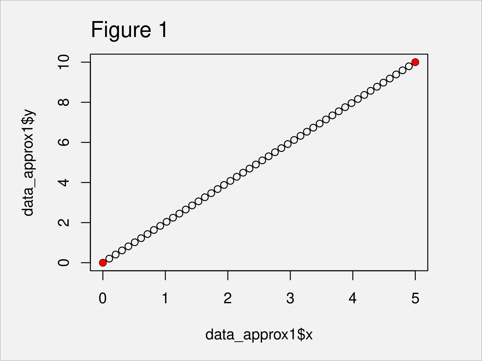
Figure 1 shows the output of the previous R syntax – We have created a scatterplot that shows the linear interpolates created by the approx function. The two original coordinates are shown in red and the interpolation points are shown in black.
Example 2: Apply approx Function to Multiple Coordinates
Example 1 has explained how to interpolate between two different data points. In this section, I’ll explain how to interpolate between multiple data points.
First, we have to create two new example vectors:
x2 <- c(0, 5, 10, 15)                # Create first vector
x2                                   # Print first vector
# [1]  0  5 10 15
y2 <- c(0, 10, 100, 1000)            # Create second vector
y2                                   # Print second vector
# [1]    0   10  100 1000
As you can see, each of our vectors consists of four integer elements.
Next, we can use the approx function as we already did in Example 1:
data_approx2 <- approx(x2, y2)       # Apply approx function
data_approx2                         # Return output of approx function
# $x
#  [1]  0.0000000  0.3061224  0.6122449  0.9183673  1.2244898  1.5306122
#  [7]  1.8367347  2.1428571  2.4489796  2.7551020  3.0612245  3.3673469
# [13]  3.6734694  3.9795918  4.2857143  4.5918367  4.8979592  5.2040816
# [19]  5.5102041  5.8163265  6.1224490  6.4285714  6.7346939  7.0408163
# [25]  7.3469388  7.6530612  7.9591837  8.2653061  8.5714286  8.8775510
# [31]  9.1836735  9.4897959  9.7959184 10.1020408 10.4081633 10.7142857
# [37] 11.0204082 11.3265306 11.6326531 11.9387755 12.2448980 12.5510204
# [43] 12.8571429 13.1632653 13.4693878 13.7755102 14.0816327 14.3877551
# [49] 14.6938776 15.0000000
#
# $y
#  [1]    0.0000000    0.6122449    1.2244898    1.8367347    2.4489796
#  [6]    3.0612245    3.6734694    4.2857143    4.8979592    5.5102041
# [11]    6.1224490    6.7346939    7.3469388    7.9591837    8.5714286
# [16]    9.1836735    9.7959184   13.6734694   19.1836735   24.6938776
# [21]   30.2040816   35.7142857   41.2244898   46.7346939   52.2448980
# [26]   57.7551020   63.2653061   68.7755102   74.2857143   79.7959184
# [31]   85.3061224   90.8163265   96.3265306  118.3673469  173.4693878
# [36]  228.5714286  283.6734694  338.7755102  393.8775510  448.9795918
# [41]  504.0816327  559.1836735  614.2857143  669.3877551  724.4897959
# [46]  779.5918367  834.6938776  889.7959184  944.8979592 1000.0000000
Let’s draw these data in a scatterplot:
plot(data_approx2$x,                 # Draw output of approx function
     data_approx2$y)
points(x2, y2,
       col = "red",
       pch = 16)

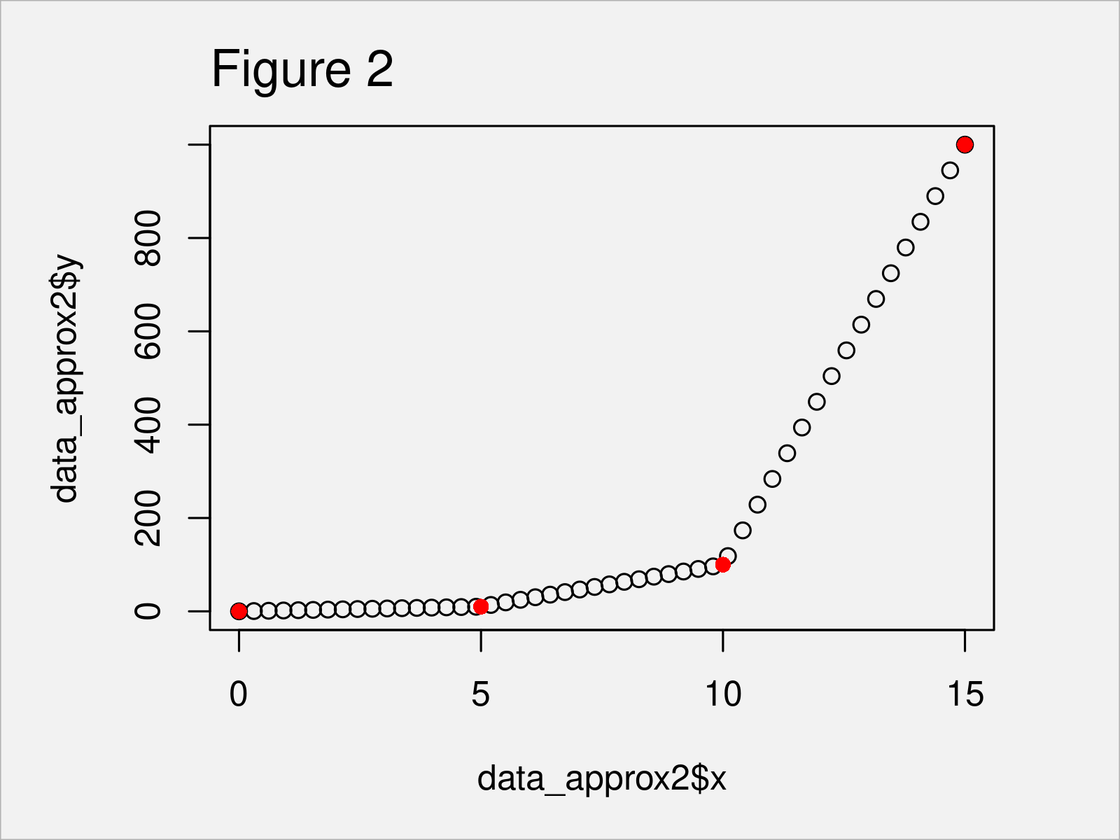
After running the previous R programming syntax the scatterplot shown in Figure 2 has been drawn. As you can see, we have linearly interpolated between multiple data points.
Example 3: Create User-Defined Interpolation Function Using approxfun
In Examples 1 and 2, I have explained how to return interpolations using the approx function.
Example 3 illustrates how to use the approxfun to construct a user-defined function that performs linear (or constant) interpolation.
Have a look at the following R code:
my_approxfun <- approxfun(x2, y2) # Apply approxfun function
By executing the previous R code, we have created our own function based on the numeric vectors created in Example 2.
We can now use this function in any way we want. For instance, we may use this function to draw a function curve:
plot(x2, y2)                         # Draw output of approxfun function
curve(my_approxfun,
      add = TRUE)

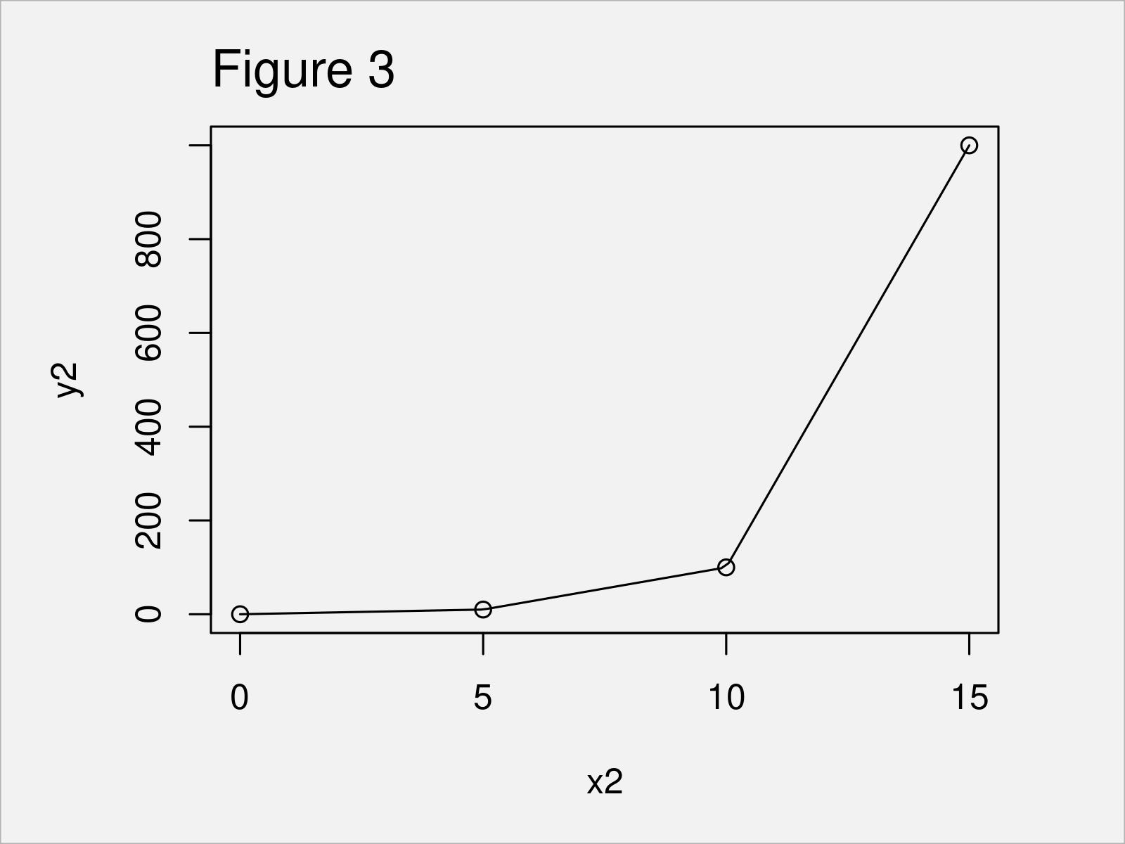
After executing the previously shown R programming syntax the point and line graphic shown in Figure 3 has been drawn. As you can see, the function curve is the same as the values shown in the plot that we have created in Example 2.
Video & Further Resources
Some time ago, I have released a video on my YouTube channel, which illustrates the topics of this tutorial. You can find the video below.
In addition, you could have a look at the related tutorials on this homepage.
- Draw Plot of Function Curve in R
- Draw Multiple Function Curves to Same Plot
- Fit Smooth Curve to Plot of Data in R
- List of R Functions
- R Programming Language
In summary: This tutorial has demonstrated how and when to use the approx and approxfun interpolation functions in the R programming language. If you have further comments or questions, let me know in the comments section.


