optim Function in R (Example)
On this page you’ll learn how to apply a general-purpose optimization using the optim function in the R programming language.
Table of contents:
So without further ado, let’s dive right in:
Creation of Example Data
The following data is used as basement for this R programming tutorial:
set.seed(93420)                         # Creating random data
x <- rnorm(500)
y <- rnorm(500) + 0.7 * x
data <- data.frame(x, y)
head(data)                              # Print head of data
#             x           y
# 1 -0.21492991 -0.06814474
# 2 -0.02217756 -0.84956484
# 3  0.55175788  0.11247758
# 4 -0.33581492 -0.86346317
# 5 -0.02489514  0.44307381
# 6 -1.44784931 -2.49701457
The previous output of the RStudio console shows the structure of our example data: It contains two numeric variables x and y.
Example: Applying optim Function in R
In this Example, I’ll explain how to use the optim function to minimize the residual sum of squares in the R programming language. First, we’ll manually create a function that computes the residual sum of squares. Please note that this function and the following R code is partly based on a tutorial that I found here.
my_function <- function(data, par) {    # Own function for residual sum of squares
  with(data, sum((par[1] + par[2] * x - y)^2))
}
Now, we can use the optim function as shown below. The par argument specifies the initial values for the parameters to be optimized over, the fn argument specifies our function, and the data argument specifies our data frame. We are storing the output of the optim function in the data object optim_output:
optim_output <- optim(par = c(0, 1),    # Applying optim
                      fn = my_function,
                      data = data)
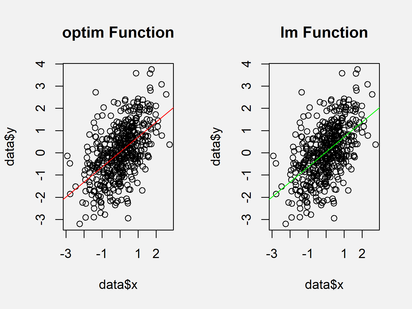
Next, we can visualize our results in a plot. For comparison, I’m going to plot our results of the optim function side-by-side with the results of a conventional linear model provided by the lm function. If we’ve done everything correctly, the output of both functions should be the same.
First, we have to specify the settings of our plot using the par function:
par(mfrow = c(1, 2)) # Setting plot parameters
Now, we can draw the results of the optim function on the left side of our graphic…
plot(data$x,                            # Plotting results of optim function
     data$y,
     main = "optim Function")
abline(optim_output$par[1],
       optim_output$par[2],
       col = "red")
…and the results of the lm function at the right side of our graphic:
plot(data$x,                            # Plotting results of lm function
     data$y,
     main = "lm Function")
abline(lm(y ~ x, data),
       col = "green")

Figure 1 shows the output of the previous R code: Both the optim and the lm functions returned the same result. In other words, our manual optimization using the optim function worked fine.
Video & Further Resources
Do you need further information on the R programming codes of this article? Then you might have a look at the following video of my YouTube channel. In the video, I’m showing the R programming codes of this tutorial:
The YouTube video will be added soon.
Furthermore, you might read the related articles of www.statisticsglobe.com:
In summary: This page showed how to apply the optim function in the R programming language. Don’t hesitate to let me know in the comments, in case you have additional questions.
Subscribe to the Statistics Globe Newsletter
Get regular updates on the latest tutorials, offers & news at Statistics Globe.
I hate spam & you may opt out anytime: Privacy Policy.
Thank you!
Welcome to the Statistics Globe newsletter. From now on, I’ll send you regular emails about statistics, data science, AI, and programming with R and Python.
I’m Joachim Schork. On this website, I provide statistics tutorials as well as code in Python and R programming.
Statistics Globe Newsletter
Get regular updates on the latest tutorials, offers & news at Statistics Globe. I hate spam & you may opt out anytime: Privacy Policy.
Thank you!
Please check your email inbox and click the confirmation link to complete your subscription. If you don’t see the email within a few minutes, please also check your spam/junk folder.


