Probability Distributions in R (Examples) | PDF, CDF & Quantile Function

This page explains the functions for different probability distributions provided by the R programming language.

In general, R provides programming commands for the probability distribution function (PDF), the cumulative distribution function (CDF), the quantile function, and the simulation of random numbers according to the probability distributions.

The naming of the different R commands follows a clear structure. See the table below for the names of all R functions:

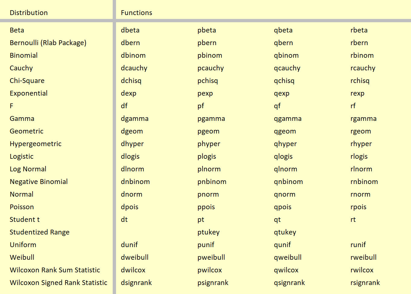
all probability distribution functions of the r programming language

Table 1: The Probability Distribution Functions in R.

Table 1 shows the clear structure of the distribution functions. The names of the functions always contain a d, p, q, or r in front, followed by the name of the probability distribution.

Hereby, d stands for the PDF, p stands for the CDF, q stands for the quantile functions, and r stands for the random numbers generation.

For instance, the normal distribution its PDF is obtained by dnorm, the CDF is obtained by pnorm , the quantile function is obtained by qnorm, and random number are obtained by rnorm.

Below, you can find tutorials on all the different probability distributions. Each tutorial contains reproducible R codes and many examples.

All Tutorials on Probability Distributions in R

Bernoulli Distribution in R (4 Examples) | dbern, pbern, qbern & rbern Functions

Beta Distribution in R (4 Examples) | dbeta, pbeta, qbeta & rbeta Functions

Binomial Distribution in R (4 Examples) | dbinom, pbinom, qbinom & rbinom Functions

Calculate Critical t-Value in R (3 Examples)

Calculate Skewness & Kurtosis in R (2 Examples)

Cauchy Density in R (4 Examples) | dcauchy, pcauchy, qcauchy & rcauchy Functions

Chi Square Distribution in R (4 Examples) | dchisq, pchisq, qchisq & rchisq Functions

Continuous Uniform Distribution in R (4 Examples) | dunif, punif, qunif & runif Functions

Exponential Distribution in R (4 Examples) | dexp, pexp, qexp & rexp Functions

F Distribution in R (4 Examples) | df, pf, qf & rf Functions

Gamma Distribution in R (4 Examples) | dgamma, pgamma, qgamma & rgamma Functions

Generate Matrix with i.i.d. Normal Random Variables in R (2 Examples)

Generate Multivariate Random Data in R (2 Examples)

Generate Random Values with Fixed Mean & Standard Deviation in R (2 Examples)

Generate Set of Random Integers from Interval in R (2 Examples)

Geometric Distribution in R (4 Examples) | dgeom, pgeom, qgeom & rgeom Functions

Half Normal Distribution in R (4 Examples)

Hypergeometric Distribution in R (4 Examples) | dhyper, phyper, qhyper & rhyper Functions

32 Comments. Leave new

Gowtham S
December 5, 2021 10:17 am

Hi, I am interested in learning how to R is being used in probability model. In most of the case I could see rolling a fair dice but incase of un-fair dice, how can it be approached. Please share me some resources for probability models using R.

Reply
- Joachim
  December 6, 2021 7:31 am
  
  Hey Gowtham,
  
  This could be simulated with the sample function. Within the sample function, you can specify probabilities for each number.
  
  Regards,
  Joachim
  
  Reply
Mohammad Yarahmadi
August 14, 2022 5:42 pm

Hello, dear Mr. Joachim Schork
I’m working on an article, I’m almost finished, now I need a series of x and y data, I want to see if they follow the generalized Rayleigh distribution (Burr type x) or not…
No matter what I do, I cannot find and run the codes in R
Thank you for your advice.

I want to do something like this

install.packages(“fitdistrplus”)
library(“fitdistrplus”)
install.packages(“VGAM”)
library(“VGAM”)
install.packages(“rmutil”)
library(“rmutil”)
######################
##########################
x=c(26,63,19,66,40,49,8,69,39,82,72,66,25,41,16,18,22,42,36,34,53,54,51,76,64,26,16,44,25,55,49,24,44,42,27,28,2)
y=c(20,18,19,85,40,49,8,71,39,48,72,62,9,3,75,18,14,42,52,34,39,7,28,64,15,48,16,13,14,11,49,24,30,2,47,28,2)
data=c(x=x,y=y)
#################################
##########################################################
hist(data)
#######################
plot(density(data))
descdist(data, boot=10000)
#################################
fnorm = fitdist(data, “norm”)
fgamma = fitdist(data, “gamma”)
flognorm = fitdist(data, “lnorm”)
fexp = fitdist(data, “exp”)
########################################
plot.legend = c(“Normal”, “Gamma”, “LogNormal”, “Exponential”)
dist.list = list(fnorm, fgamma, flognorm, fexp)
denscomp(dist.list,legendtext = plot.legend)
cdfcomp(dist.list, legendtext = plot.legend)
###########################################
gofstat(dist.list , fitnames=plot.legend)
ks.test(data, pexp, fexp$estimate[1], fexp$estimate[2])
ks.test(data, pnorm, fnorm$estimate[1], fnorm$estimate[2])
ks.test(data, plognorm, flognorm$estimate[1], flognorm$estimate[2])
ks.test(data, pgamma, fgamma$estimate[1], fgamma$estimate[2])

Reply
- Joachim
  August 15, 2022 8:08 am
  
  Hey Mohammad,
  
  I’m not an expert on the generalized Rayleigh distribution. However, I have just tried to run your code, and it seems to work fine. Could you specify your problem in some more detail?
  
  Regards,
  Joachim
  
  Reply
David Bartley
May 5, 2023 7:19 am

Within Mathematica, CDF and quantile are easily computed, given a user-defined PDF (in addition to the common distributions). Are there similar established routines in R, or must I use R’s integrate for CDF and an inversion routine for quantile?

Reply
- Cansu (Statistics Globe)
  May 5, 2023 3:44 pm
  Hello David,
  
  It looks like you can use the integrate() function to find the cdf of the user-defined pdf. Then use the uniroot() function to find the quantiles. See the example code below.
  custom_pdf <- function(x) { return(3 * x^2) # Example: x^3 distribution from 0 to 1 } # Compute the CDF custom_cdf <- function(x) { result <- integrate(custom_pdf, lower = 0, upper = x) return(result$value) } # Compute the quantile custom_quantile <- function(p) { result <- uniroot(function(x) custom_cdf(x) - p, interval = c(0, 1)) return(result$root) } # Test the functions cdf_value <- custom_cdf(0.5) quantile_value <- custom_quantile(0.5)
  This code defines a custom PDF for x^3 distribution, computes the CDF at x = 0.5, and finds the quantile at p = 0.5.
  Reply
David Bartley
May 7, 2023 2:23 pm

Thanks so much Cansu,

However, with:

pdf = -1 && x<=+1) return((1/4)*(1-x)^3) else return(0) }

When I compute pdf(-2.10), pdf(-2), pdf(-1.5), pdf(.5), etc. pdf is computed correctly.

But your program:

cdf <- function(x) { result = -1 && x <= +1 : 'length = 101' in coercion to 'logical(1)'

Thanks,

David

Reply
- Cansu (Statistics Globe)
  May 8, 2023 7:55 am
  
  Hello,
  
  Could you please share how you defined your cdf?
  
  Regards,
  Cansu
  
  Reply
David Bartley
May 8, 2023 9:55 am

Cansu,

I don’t know how my message to you became so entirely corrupted. Let me start over. First of all, the probability distribution function pdf is defined as:

pdf = -1 && x= -1 && x 0.

cdf may be defined as:

cdf <- function(x) {
result 0.

My questions:

(1) Why the original error message?

(2) Is there a simple way to plot from x = −1 to x = 1?

Thanks,

David

Reply
David Bartley
May 8, 2023 9:59 am

Cansu,

Again, my message is corrupted. There is something wrong with this method of messaging. Can I email you my question somehow?

David

Reply
- Cansu (Statistics Globe)
  May 8, 2023 10:06 am
  
  Hello David,
  
  Can you describe your pdf in words then I can try to help. What kind of function it is, etc.?
  
  Regards,
  Cansu
  
  Reply
David Bartley
May 8, 2023 11:00 am

Cansu,

This message system is not working. Could you send me an email address so as to send you my questions?

Thanks,

David

Reply
- Cansu (Statistics Globe)
  May 8, 2023 11:14 am
  
  Hello David,
  
  I am so sorry, I don’t share my private email. It is strange that the messaging system doesn’t work for you. Because I have been answering comments for months in the comment sections, and no one has mentioned about that. If you mean that you can not see your message after posting it, then it is totally normal. Because the messages are posted after our approval to avoid scams.
  
  Regards,
  Cansu
  
  Reply
David Bartley
May 8, 2023 11:34 am

Cansu,

Maybe my browser is not working correctly, so let me switch to another.

First of all, the probability distribution function pdf is defined as:

pdf = -1 && x= -1 && x 0.

cdf may be similarly fixed with “Vectorize” as:

cdf <- function(x) {
result 0.

My questions:

(1) Why the original error message?
(2) Is there a simple way to plot from x = −1 to x = 1?

Thanks,

David

Reply
David Bartley
May 8, 2023 11:36 am

No. For some reason, the definition for pdf, etc. becomes gibberish. I’m giving up for now.

David

Reply
- Cansu (Statistics Globe)
  May 8, 2023 11:43 am
  
  Hey David!
  
  Could you please try to embed your code script in the following HTML:
  
  <pre lang="csharp">XXXXXXXXXX_R_CODE_XXXXXXXXXX</pre>
  
  I hope it helps.
  
  Regards,
  Cansu
  
  Reply

David Bartley

May 9, 2023 8:03 am

Cansu,

Try reading my questions saved at Dropbox:

https://www.dropbox.com/s/eziacwi7jzi3j8f/To%20Cansu.rtf?dl=0https://www.dropbox.com/s/eziacwi7jzi3j8f/To%20Cansu.rtf?dl=0

Thanks,

David

Cansu (Statistics Globe)

May 9, 2023 9:36 am

Hello David,

The problem is you don’t let the function take multiple values; that is the first problem. As you figured out, you need a vector as an input. Also, you should modify the if statement a bit since the loop will be terminated when you use return(). You should initialize a results vector, append each result one by one, and return it. See below.

pdf <- function(x) {                   # define function 
  result <- numeric(length(x))
 
  for (i in 1:length(x)) {
    if (x[i] >= -1 && x[i] <= 1) {
      result[i] <- (1 / 4) * (1 - x[i])^3
    } else {
      result[i] <- 0
    }
  }
 
  return(result)
}
 
y <- seq(-1,1,0.01)                     # define input 
values<-pdf(y)                          # define output 
values[1:5]                             # print first 5 values 
# [1] 2.000000 1.970150 1.940598 1.911343 1.882384
 
plot(values) # plot function

But there is a simple way to plot a function using the stat_function layer of ggplot2. See below.

library(ggplot2)                        # do all using ggplot2 library 
ggplot(data.frame(values = c(-1, 1)), aes(values)) +
  stat_function(fun = pdf, color = "blue", size = 1)

I hope these solutions help.

Regards,
Cansu

David Bartley
May 10, 2023 1:27 am

Cansu,

Thanks for answering.

No, there is no loop. Any looping would be done within the plot routine and should be entirely invisible to the user. Also, the error message after plot() was really peculiar, giving no clue as to its resolution. In fact, resolution could possibly be done within the plot() routine itself. This must be a recurring problem within R.

I do not have ggplot2. Does plot(), have options for specifying the frame range (e.g., −1 to +1 in my sample case)? The plotting does work correctly for x = 0 to 1 as long as “Vectorize” is used.

This is all really cumbersome and could make addressing more serious applications next to impossible. I’m guessing that R is simply not set up to do such calculations and is mainly for analyzing a variety of datasets.

David

Reply
- Cansu (Statistics Globe)
  May 10, 2023 7:31 am
  Hello David,
  
  Sorry, I shared the wrong code for the first solution. Please see the following for plotting via plot().
  pdf <- function(x) { # define function result <- numeric(length(x)) for (i in 1:length(x)) { if (x[i] >= -1 && x[i] <= 1) { result[i] <- (1 / 4) * (1 - x[i])^3 } else { result[i] <- 0 } } return(result) } y <- seq(-1,1,0.01) # define input values<-pdf(y) # define output values[1:5] # print first 5 values # [1] 2.000000 1.970150 1.940598 1.911343 1.882384 plot(values) # plot function
  Also, you can install the ggplot2 package easily as follows.
  install.packages("ggplot2") library(ggplot2) # do all using ggplot2 library ggplot(data.frame(values = c(-1, 1)), aes(values)) + stat_function(fun = pdf, color = "blue", size = 1)
  I think it is easier to plot such functions using ggplot2. Sorry for the inconvenience again.
  
  Regards,
  Cansu
  Reply
David Bartley
May 12, 2023 8:29 am

Cansu,

OK. Here’s my question:

Suppose you define an array y as you did:

y <- seq(-1,1,0.01)

Then a common function like sin() in R with argument y returns an array:

sin(y)

Now then, suppose I define a function pdf via the simple expression:

pdf = -1 && x= -1 && x <= +1 : 'length = 201' in coercion to 'logical(1)'

Why? Why must we resort to your complicated definition of pdf?

David

Reply
David Bartley
May 12, 2023 8:37 am

Again, on replying to you, 4 lines of my reply were strangely deleted. The end should read:

Now then, suppose I define a function pdf via the simple expression:

pdf = -1 && x= -1 && x <= +1 : 'length = 201' in coercion to 'logical(1)'

Why? Why must we resort to your complicated definition of pdf?

David

Reply
David Bartley
May 12, 2023 8:39 am

Again, lines deleted.

Reply
David Bartley
May 12, 2023 8:41 am

Maybe there’s an invisible character in my text that throws the comment box off.

Reply
David Bartley
May 12, 2023 8:52 am

Anyway, my earlier simple definition of pdf, just like sin, computes a value for any individual argument x (e.g., -.2,0,.4, etc.).

However, unlike sin, my pdf with argument y, pdf(y), does not return an array, but gives the peculiar error:

Error in x >= -1 && x <= +1 : 'length = 201' in coercion to 'logical(1)'

Why? Why must we resort to your complicated definition of pdf?

David

Reply
David Bartley
May 12, 2023 9:19 am

Cansu,

I finally figured out how to use “plot”. With my simpler scalar definition of pdf, as I mentioned earlier, plot(Vectorize(pdf) correctly plots for x > 0. At last, I found that plot(Vectorize(pdf, −2, 2) also correctly plots for −2 < x = -1 && x <= +1 : 'length = 201' in coercion to 'logical(1)'

and found out that this sort of problem began with version 4.2.1

David

Reply
David Bartley
May 12, 2023 9:27 am

Typos: Should be plot(Vectorize(pdf)) and plot(Vectorize(pdf), −2, 2)

Reply
David Bartley
May 12, 2023 5:12 pm

Cansu,

Now here is something interesting. Using abs(x)= -1 && x<=+1) as condition does not require Vectorize for plot or other functions.

For example, try:

pdf<-function(x) { ifelse(abs(x)= -1 && x <= +1 : 'length = 101' in coercion to 'logical(1)'

does not appear.

David

Reply
David Bartley
May 12, 2023 5:25 pm

Again, the Comment box deleted lines. Here is what I was just now trying to send you:

https://www.dropbox.com/s/ybe31awu7bsnj49/To%20Cansu%202.rtf?dl=0

David

Reply
- Cansu (Statistics Globe)
  May 15, 2023 6:51 am
  
  Hello David,
  
  I understand that you managed to use the function the way you liked it in the end. I am happy to hear that. If you have any questions regarding the provided solution by me, let me know.
  
  Regards,
  Cansu
  
  Reply
David Bartley
May 18, 2023 7:43 am

Cansu,

Please see thank you note:

https://www.dropbox.com/s/7ufpxmur9aabp2e/To%20Cansu%203.rtf?dl=0

You might be located in the UK somewhere, since you’re at work while I’m night-owling!

David

Reply
- Cansu (Statistics Globe)
  May 19, 2023 10:58 am
  
  Appreciated.
  
  Regards,
  Cansu
  
  Reply

Probability Distributions in R (Examples) | PDF, CDF & Quantile Function

All Tutorials on Probability Distributions in R

32 Comments. Leave new

Leave a Reply Cancel reply